So far, we’ve introduced you to R and RStudio, explained the basics of setting up a project in R, and talked about R packages. But the real reason you want to use R is to do data analysis or make charts. To do either of those things, you’ve got to get your data into R! There are several approaches to loading data into R, but the most straightforward (and most common) is to read data in from CSV, Excel, or other file types.
RStudio project organization
Before we dive into importing data, let’s take a quick detour and talk about project organization. As discussed earlier, whenever you are working in R, we strongly recommend that you use RStudio Projects to keep your files organized and self-contained. Whenever possible, you should keep your code, data, notes, and output for a single project all in the same folder structure.
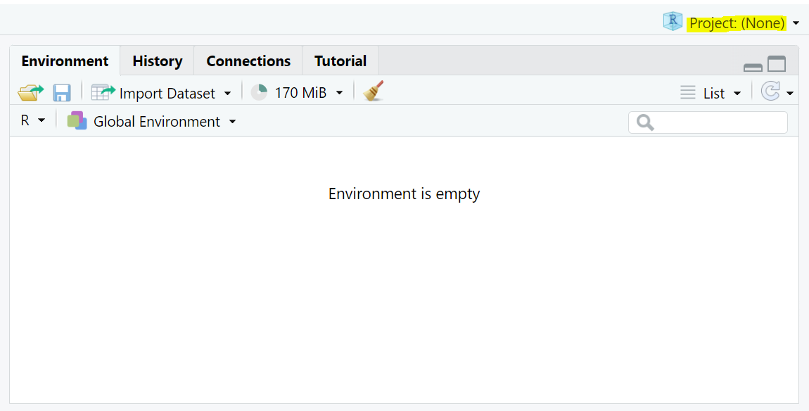
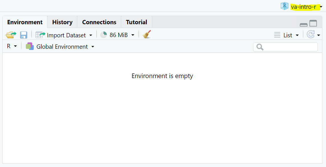
If you’re following along on your computer, look in the upper right corner of RStudio. Make sure you see the name of an active project now and whenever you are coding in R.
Sad (Not so good)
Happy (Great!)
Within a data analysis project, we recommend, at minimum, the following folders:
R: contains all R script files
data: contains all data files
output: contains saved artifacts, such as plots, tables, or regression results
Reading data in from a CSV file
One of the most common file formats to store and share data is the CSV (comma-separated values) file. This is a plain text file that uses commas to separate values and line breaks to separate rows. For this example, we’ll use a CSV file called nps-admissions.csv. To follow along with the examples here, right click on this link and save the nps-admissions.csv file into the data folder of your RStudio project.
Throughout this course, we’ll be working with publicly available data from the Bureau of Justice Statistics National Prisoner Statistics (NPS) Program. NPS data is collected annually by BJS from state corrections departments and contains aggregate counts of people incarcerated, people admitted, and people released, as well as demographic details about the prison population, types of admissions, reasons for releases, and other details of state prison operations. We’ve created simplified versions of the NPS dataset for teaching purposes. You can download the full NPS dataset from the National Archive of Criminal Justice Data.
In the upper left corner of RStudio, click File > New File > R Script to open a blank script (alternatively, use the keyboard shortcut Ctrl + Shift + N). The first thing we need to do is attach the tidyverse package, because we’re going to be using functionality from that package to import the CSV file. Type library(tidyverse)your new R script. To execute this line of code, press Ctrl + Enter. This will “send” the code from your script (in the Source pane) to the Console. You’ll see the results of running that line of code printed in the Console.
library(tidyverse)
── Attaching core tidyverse packages ──────────────────────── tidyverse 2.0.0 ──
✔ dplyr     1.1.4     ✔ readr     2.1.5
✔ forcats   1.0.0     ✔ stringr   1.5.1
✔ ggplot2   3.5.1     ✔ tibble    3.2.1
✔ lubridate 1.9.4     ✔ tidyr     1.3.1
✔ purrr     1.0.2
── Conflicts ────────────────────────────────────────── tidyverse_conflicts() ──
✖ dplyr::filter() masks stats::filter()
✖ dplyr::lag()    masks stats::lag()
ℹ Use the conflicted package (<http://conflicted.r-lib.org/>) to force all conflicts to become errors
Next, we’re going to read the NPS admissions data in and create a new dataset in R called nps_admit. Type the following into your script and then execute it by pressing Ctrl + Enter:
nps_admit <-read_csv("data/nps-admissions.csv")
You won’t see any output printed in the Console, but you’ll see there is a new object in the Environment tab in the upper right pane. Click on nps_admit in the Environment to view the data.
Exploring datasets
Another way to explore the data is by typing the name of the new dataset (nps_admit) in your script and running the code with Ctrl + Enter:
nps_admit
# A tibble: 11,475 × 6
    year state_name state_abbr adm_type           m     f
   <dbl> <chr>      <chr>      <chr>          <dbl> <dbl>
 1  1978 Alabama    AL         adm_total       2631   184
 2  1978 Alabama    AL         adm_new_commit  2115   148
 3  1978 Alabama    AL         adm_viol_new       0     0
 4  1978 Alabama    AL         adm_viol_tech    150     5
 5  1978 Alabama    AL         adm_oth          155    31
 6  1979 Alabama    AL         adm_total       2596   223
 7  1979 Alabama    AL         adm_new_commit  2314   178
 8  1979 Alabama    AL         adm_viol_new       0     0
 9  1979 Alabama    AL         adm_viol_tech     68     2
10  1979 Alabama    AL         adm_oth          214    43
# ℹ 11,465 more rows
Let’s take a closer look at the output here. When we print the dataset in the Console, we see a preview of the first 10 rows of the dataset along with some additional useful information. For instance, we can see that there are 11,745 rows and 6 columns. Additionally, printed below each of the column names is an abbreviation indicating the type of data contained in the column. In this case, year, m, and f are double or numeric columns (indicated by <dbl>) and state_name, state_abbr, and adm_type are character or string columns (indicated by <chr>). We’ll talk in more depth about data types in the Lesson 7.
There’s one other useful approach to start exploring what is in a dataset. For this, we’re going to use the count() function, which takes a column in a dataset and counts the number of times each value in the column appears. In this case, let’s count the adm_type column of the nps_admit dataset and see what the possible values are and how many times they appear.
There are five different admission types in this dataset and each of them appears 2,295 times. We’ll discuss count() in more detail later, but for now, just know that it’s a very useful tool for quickly summarizing a column in a dataset. In our Data Quality Fundamentals course, we will talk more about how to assess your data and understand if you are working with the right dataset for your project, if you need to adjust an analysis because of data quality, etc. For now, note that good analysts almost always run count as soon as they import data.
You can also view the entire dataset by running View(nps_admit). This will open the dataset in a new tab of the Source pane that you can browse, sort, and filter.
Reading data in from Excel files
The process of reading data from Excel workbooks is very similar to reading CSV files. To do this, you’ll first need to attach the readxl package (if you haven’t already installed it, you’ll need to install first). Then instead of read_csv(), use read_excel(). To follow along with our examples, download nps-releases.xlsx by right clicking on this link and save it to the data folder of your project. Then run the following code to create a new dataset called nps_release that contains the data in the releases Excel file.