library(tidyverse)

nps_admit <- read_csv(path = "data/nps-admissions.csv")Lesson 7: Coding Basics
Introduction
In the previous lessons, you ran code that imports data, explores data, and makes plots, but you haven’t yet learned the core elements of the code. In this lesson, you’ll learn some coding basics that will help you get a handle on foundational elements of programming (writing code) in R including object assignment, functions, data frames, and data types.
Code building blocks
Using the example from Lesson 5 in which you imported National Prisoner Statistics data from a CSV file, and you’ll now learn the elements of that code.
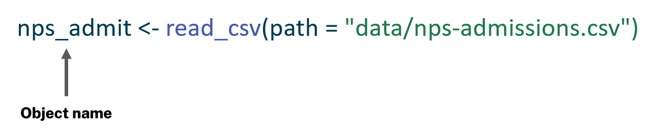
Object names
The first part of the code, nps_admit is the name of the new object you are creating. Objects in R can be many different things, such as data frames, vectors, or lists. But the basic idea is that an object is a named “thing” that is stored in R memory that you can refer to by its name.
It’s true—naming things is harder than it seems!
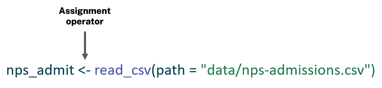
Assignment
The next part of the code, <-, is the assignment operator; this is how you create new objects. The left side of the assignment operator is the name of the object you are creating, and the right side is the value that will be assigned to that name.
The generic form of assignment in R looks like this:
object_name <- valueFor example, you can create a new object called x and assign the value of x to be 3 times 4.
x <- 3 * 4Note that when you create a new object, its value is not printed. To view the value of an object, type its name in the console and press Enter.
x[1] 12Now that you’ve assigned a value to the x object, you can refer to that object by name later in the script. Here, divide x by 4.
x / 4[1] 3You could also create a second object, y, and divide x by y.
y <- 6
x / y
[1] 2There is a useful RStudio feature that displays all the assigned objects in your R session. In the upper right pane of RStudio, you should have an Environment tab that shows basic information about objects. As you create new objects, they will be added here. After running the code to this point in the lesson, this is what the Environment tab should look like:
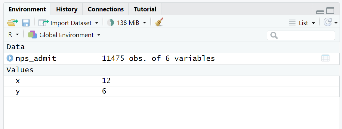
The History tab contains a record of all the commands that have been executed in the Console. The Connections and Tutorial tabs are less commonly used.
Functions
Returning to the example of importing data, the value you are assigning to nps_admit is the output of a function. A function is a block of code that is stored and executed when you run or “call” the function. To use a function, you type its name and then one or more arguments and argument values within parentheses.
Generically, calling functions in R follows this form:
function_name(argument1 = argument_value1, argument2 = argument_value2, ...)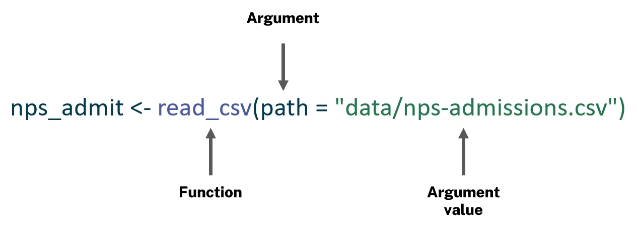
Here, the function you are calling is read_csv() and the argument value is the path to the CSV file, "data/nps-admissions.csv".
Arguments
R functions can have one or more arguments that affect how a function operates. For instance, the rep() function in R replicates or repeats values a certain number of times depending on the argument values.
To see what arguments a function takes, use the built-in documentation for a function. Type a question mark before the name of a function and press Enter in the Console to open the help page for that function in RStudio.
?repIn the code below, the function is rep(), its arguments are x and times, and the argument values are "hello" and 2.
rep(x = "hello", times = 2)[1] "hello" "hello"You can run this again and modify the arguments to get a different result.
rep(x = "goodbye", times = 4)[1] "goodbye" "goodbye" "goodbye" "goodbye"Data frames
Data frames are one of the most used data structures in R, especially when doing data analysis and visualization. You can think of a data frame like an Excel worksheet: a table that contains data in columns and rows. When you do data analysis in R, you’ll usually be working with one or more data frames to filter rows, create new columns, aggregate or summarize data, or join multiple data frames. Data frames in R have special rules; each column must (1) have the same number of rows and (2) contain the same type of data in every row of that column.
Data manipulation techniques will be covered in future lessons.
In fact, you’ve already seen data frames in previous lessons! The nps_admit dataset that you created by reading in data from a CSV file is a data frame with 11,475 rows and 6 columns.
You may also see data frames referred to as tibbles; this is confusing, but they are essentially the same thing.
nps_admit# A tibble: 11,475 × 6
year state_name state_abbr adm_type m f
<dbl> <chr> <chr> <chr> <dbl> <dbl>
1 1978 Alabama AL adm_total 2631 184
2 1978 Alabama AL adm_new_commit 2115 148
3 1978 Alabama AL adm_viol_new 0 0
4 1978 Alabama AL adm_viol_tech 150 5
5 1978 Alabama AL adm_oth 155 31
6 1979 Alabama AL adm_total 2596 223
7 1979 Alabama AL adm_new_commit 2314 178
8 1979 Alabama AL adm_viol_new 0 0
9 1979 Alabama AL adm_viol_tech 68 2
10 1979 Alabama AL adm_oth 214 43
# ℹ 11,465 more rowsData types
You can have numbers in one column and text in another column, but not a single column that mixes numbers and text. There are several data types in R; the ones you’ll see most frequently are character and numeric.
Other R data types are integer, logical, complex, and raw.
Characters or strings contain text and can be used for categorical variables like facility, race, or name, while numeric variables store numbers.
In the nps_admit data frame you’ve been working with, there are 6 columns. Three of the columns are characters and three are numeric. When you print a data frame in the console, the data types are displayed below the column names.
Technically, this only happens when you print a tibble.
nps_admit# A tibble: 11,475 × 6
year state_name state_abbr adm_type m f
<dbl> <chr> <chr> <chr> <dbl> <dbl>
1 1978 Alabama AL adm_total 2631 184
2 1978 Alabama AL adm_new_commit 2115 148
3 1978 Alabama AL adm_viol_new 0 0
4 1978 Alabama AL adm_viol_tech 150 5
5 1978 Alabama AL adm_oth 155 31
6 1979 Alabama AL adm_total 2596 223
7 1979 Alabama AL adm_new_commit 2314 178
8 1979 Alabama AL adm_viol_new 0 0
9 1979 Alabama AL adm_viol_tech 68 2
10 1979 Alabama AL adm_oth 214 43
# ℹ 11,465 more rowsUnder state_name, state_abbr, and adm_type you should see <chr>, which indicates these are character columns. And under year, m, and f you should see <dbl>, which indicates these are numeric columns.
dbl is short for “double,” a column type that allows you to store decimal or real numbers.
It’s important to be aware of data types because you might run into some surprising issues if data you expect to be numbers are stored as characters or vice versa.
Code comments
One last code basic that you should know about is code comments. Comments are text you write in R scripts that are ignored by R but meant to be read by people. These comments are useful for describing what code does and why an analyst has made particular choices. When someone else is checking your work or replicating it years from now, comments will help them understand the choices you made. It will also help you remember what each section of the code does.
For example, you might add the following comment to your script so that someone who’s looking at this code can quickly understand that the next line reads in National Prisoner Survey data. Without the comment, someone might not know what nps stands for. You can add comments anywhere in a script by starting a line with # and typing the text of your comment.
# read in bjs national prisoner survey admissions data
nps_admit <- read_csv(path = "data/nps-admissions.csv")
There are lots of approaches to commenting and documenting code, but Hadley Wickham’s advice from R for Data Science is useful to keep in mind:
As the code you’re writing gets more complex, comments can save you (and your collaborators) a lot of time figuring out what was done in the code. . . .For data analysis code, use comments to explain your overall plan of attack and record important insights as you encounter them. There’s no way to re-capture this knowledge from the code itself.