# A tibble: 4 × 5
  facility    q1    q2    q3    q4
  <chr>    <dbl> <dbl> <dbl> <dbl>
1 North     1500  1600  1550  1450
2 East      2100  2200  2350  2450
3 South     1200  1000  1050  1150
4 West 3500 3600 3400 3250Lesson 13: Reshape Data
Introduction
An important task of data cleaning or wrangling is structuring datasets in consistent ways that make them easy to analyze. The conceptual representation of this consistent structure is called tidy data. This lesson discusses and describes the principles of tidy data and shows examples of how to convert data into a tidy format by reshaping data. Once you’re able to identify tidy data and store your data using these principles, you’ll be able to analyze your data efficiently using tools from the tidyverse R package.
Tidy data
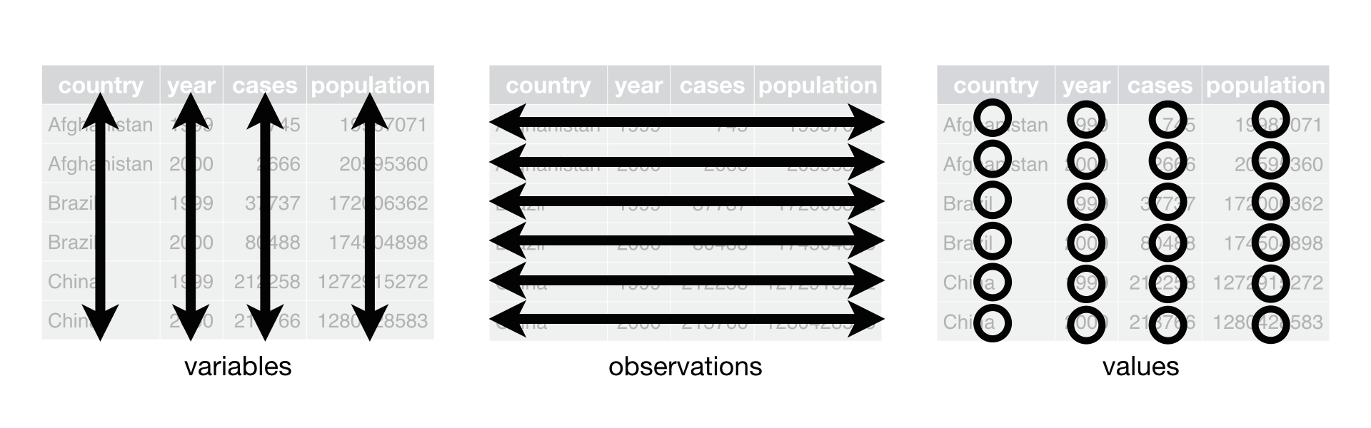
The same data can be organized in multiple ways—so tidy data proposes a system to define a tidy dataset. The tidy data concept was developed by Hadley Wickham, a well-known developer of many R packages, including the tidyverse. There are three rules that describe a tidy dataset:
Tidy data
- Each variable is a column; each column is a variable.
- Each observation is a row; each row is an observation.
- Each value is a cell; each cell is a single value.
Imagine your state had four correctional facilities and you had quarterly population data for each facility. The dataset might look something like this, where there is a single column for facility and four columns for quarter (q1, q2, q3, and q4):
This may be a good representation of the data for a warden to read in a report, but it’s not ideal for working with in R, because it does not follow tidy data principles. In particular, there are columns for q1, q2, q3, and q4. These columns aren’t variables, but rather are observations of facility population at four different points in time. To make this dataset tidy, you need a single column for population and you need to make each quarter into a row. The tidy version of this dataset looks like this:
# A tibble: 16 × 3
   facility quarter population
   <chr>    <chr>        <dbl>
 1 North    q1            1500
 2 North    q2            1600
 3 North    q3            1550
 4 North    q4            1450
 5 East     q1            2100
 6 East     q2            2200
 7 East     q3            2350
 8 East     q4            2450
 9 South    q1            1200
10 South    q2            1000
11 South    q3            1050
12 South    q4            1150
13 West     q1            3500
14 West     q2            3600
15 West     q3            3400
16 West     q4            3250
Pivoting data
The core functions you use in R to turn untidy data into tidy data are the pivot_() family of functions from the tidyr package. These functions pivot or reshape data from wide to long format or from long to wide format, depending on which restructuring is needed.
tidyr is part of the tidyverse, so you don’t need to attach it separately.
Wide to long
Most datasets that you encounter in the wild that are untidy are too wide. In other words, there are columns that should be rows. To make a dataset like this tidy, you need to increase the number of rows and decrease the number of columns. The quarterly population data above is an example of untidy data that needs to be pivoted to a longer format to be tidy.
Another dataset that should be made longer to be tidy is the NPS releases dataset that you’ve been working with throughout this course. Read in nps-releases.xlsx and print the data frame with the following code:
library(tidyverse)
library(readxl)

nps_release <- read_excel("data/nps-releases.xlsx")
nps_releasenps_release# A tibble: 4,590 × 8
year state_name state_abbr sex rel_total rel_uncond rel_cond rel_oth
<dbl> <chr> <chr> <chr> <dbl> <dbl> <dbl> <dbl>
1 1978 Alabama AL m 2823 1070 1485 252
2 1978 Alabama AL f 161 46 92 20
3 1979 Alabama AL m 2790 723 1777 272
4 1979 Alabama AL f 215 33 174 8
5 1980 Alabama AL m 3264 524 2173 552
6 1980 Alabama AL f 188 24 147 16
7 1981 Alabama AL m 2973 520 1695 746
8 1981 Alabama AL f 221 20 137 63
9 1982 Alabama AL m 2919 1097 1451 349
10 1982 Alabama AL f 172 44 118 10
# ℹ 4,580 more rowsNotice that the four columns that begin with rel are observations rather than variables. These columns represent different release types, and within them are the number of releases of that type for each year, state, and sex. To make this dataset tidy, you need to make the dataset longer so that there is one column for release type and one column for number of releases. To do this, use the pivot_longer() function and specify the names of the columns that you want to turn into rows:
nps_release |>
  pivot_longer(cols = c(rel_total, rel_uncond, rel_cond, rel_oth))
# A tibble: 18,360 × 6
year state_name state_abbr sex name value
<dbl> <chr> <chr> <chr> <chr> <dbl>
1 1978 Alabama AL m rel_total 2823
2 1978 Alabama AL m rel_uncond 1070
3 1978 Alabama AL m rel_cond 1485
4 1978 Alabama AL m rel_oth 252
5 1978 Alabama AL f rel_total 161
6 1978 Alabama AL f rel_uncond 46
7 1978 Alabama AL f rel_cond 92
8 1978 Alabama AL f rel_oth 20
9 1979 Alabama AL m rel_total 2790
10 1979 Alabama AL m rel_uncond 723
# ℹ 18,350 more rowsThe new name column contains the release types, and the new value column contains the number of releases. Notice that the wide dataset contains 4,590 rows and 8 columns, whereas the long version of this same data contains 18,360 rows and 6 columns. The figure below illustrates what happens in this transformation as the columns become rows.
You can improve the pivoting code above by specifying descriptive names for the new columns rather than the default name and value. In this case, call the names column release_type and the value column n_releases.
nps_release |>
  pivot_longer(
    cols = c(rel_total, rel_uncond, rel_cond, rel_oth),
    names_to = "release_type",
    values_to = "n_releases"
    )
# A tibble: 18,360 × 6
year state_name state_abbr sex release_type n_releases
<dbl> <chr> <chr> <chr> <chr> <dbl>
1 1978 Alabama AL m rel_total 2823
2 1978 Alabama AL m rel_uncond 1070
3 1978 Alabama AL m rel_cond 1485
4 1978 Alabama AL m rel_oth 252
5 1978 Alabama AL f rel_total 161
6 1978 Alabama AL f rel_uncond 46
7 1978 Alabama AL f rel_cond 92
8 1978 Alabama AL f rel_oth 20
9 1979 Alabama AL m rel_total 2790
10 1979 Alabama AL m rel_uncond 723
# ℹ 18,350 more rowsAdditionally, you can simplify the code by using the starts_with() select helper to select all the columns that start with rel rather than typing each of them out.
See Lesson 9 for more detail about select helpers.
nps_release |>
  pivot_longer(
    cols = starts_with("rel"),
    names_to = "release_type",
    values_to = "n_releases"
    )
# A tibble: 18,360 × 6
year state_name state_abbr sex release_type n_releases
<dbl> <chr> <chr> <chr> <chr> <dbl>
1 1978 Alabama AL m rel_total 2823
2 1978 Alabama AL m rel_uncond 1070
3 1978 Alabama AL m rel_cond 1485
4 1978 Alabama AL m rel_oth 252
5 1978 Alabama AL f rel_total 161
6 1978 Alabama AL f rel_uncond 46
7 1978 Alabama AL f rel_cond 92
8 1978 Alabama AL f rel_oth 20
9 1979 Alabama AL m rel_total 2790
10 1979 Alabama AL m rel_uncond 723
# ℹ 18,350 more rowsLastly, the release type rel_total is the total number of releases, so including that row in the longer version of the releases data frame risks double counting releases. Before pivoting this dataset, the rel_total column represented the total number of releases, not a disaggregation like rel_uncond, rel_cond, and rel_oth. So for this tidied version, remove the rel_total row and save this data frame as nps_release_tidy.
nps_release_tidy <- nps_release |>
  pivot_longer(
    cols = starts_with("rel"),
    names_to = "release_type",
    values_to = "n_releases"
    ) |>
  filter(release_type != "rel_total")

nps_release_tidy
# A tibble: 13,770 × 6
year state_name state_abbr sex release_type n_releases
<dbl> <chr> <chr> <chr> <chr> <dbl>
1 1978 Alabama AL m rel_uncond 1070
2 1978 Alabama AL m rel_cond 1485
3 1978 Alabama AL m rel_oth 252
4 1978 Alabama AL f rel_uncond 46
5 1978 Alabama AL f rel_cond 92
6 1978 Alabama AL f rel_oth 20
7 1979 Alabama AL m rel_uncond 723
8 1979 Alabama AL m rel_cond 1777
9 1979 Alabama AL m rel_oth 272
10 1979 Alabama AL f rel_uncond 33
# ℹ 13,760 more rowsWhy tidy?
Now that you’ve done all that tidying, what can you do with this tidy dataset that you couldn’t do with the original? First, you can group by year, state, and release type and calculate the total number of releases by type (rather than by sex in the original dataset).
nps_release_tidy |>
  group_by(year, state_name, release_type) |>
  summarize(n_releases = sum(n_releases)) |>
  ungroup()
# A tibble: 6,885 × 4
year state_name release_type n_releases
<dbl> <chr> <chr> <dbl>
1 1978 Alabama rel_cond 1577
2 1978 Alabama rel_oth 272
3 1978 Alabama rel_uncond 1116
4 1978 Alaska rel_cond 235
5 1978 Alaska rel_oth 87
6 1978 Alaska rel_uncond 0
7 1978 Arizona rel_cond 1305
8 1978 Arizona rel_oth 335
9 1978 Arizona rel_uncond 38
10 1978 Arkansas rel_cond 1435
# ℹ 6,875 more rowsRemember to ungroup() after you use group_by().
Alternately, you could do the same summarization but instead of by state, do it for the entire United States by not including state_name as a grouping variable.
nps_release_tidy |>
  group_by(year, release_type) |>
  summarize(n_releases = sum(n_releases)) |>
  ungroup()
# A tibble: 135 × 3
year release_type n_releases
<dbl> <chr> <dbl>
1 1978 rel_cond 98040
2 1978 rel_oth 15658
3 1978 rel_uncond 21756
4 1979 rel_cond 106693
5 1979 rel_oth 17053
6 1979 rel_uncond 22261
7 1980 rel_cond 114700
8 1980 rel_oth 16452
9 1980 rel_uncond 22268
10 1981 rel_cond 117984
# ℹ 125 more rowsFrom this dataset, the next logical question is what percentage of all releases in each year were of each type? Now that the data is in a tidy format, this is a straightforward calculation. Group by year and instead of summarizing to aggregate, use mutate to add a new column that is the percentage of all releases in each year.
releases_us <- nps_release_tidy |>
  group_by(year, release_type) |>
  summarize(n_releases = sum(n_releases)) |>
  ungroup() |>
  group_by(year) |>
  mutate(pct_releases = n_releases / sum(n_releases)) |>
  ungroup()

releases_us
# A tibble: 135 × 4
year release_type n_releases pct_releases
<dbl> <chr> <dbl> <dbl>
1 1978 rel_cond 98040 0.724
2 1978 rel_oth 15658 0.116
3 1978 rel_uncond 21756 0.161
4 1979 rel_cond 106693 0.731
5 1979 rel_oth 17053 0.117
6 1979 rel_uncond 22261 0.152
7 1980 rel_cond 114700 0.748
8 1980 rel_oth 16452 0.107
9 1980 rel_uncond 22268 0.145
10 1981 rel_cond 117984 0.729
# ℹ 125 more rowsFrom here, the next step is to create a couple of quick plots to show both the number of releases and percentage of releases by release type over time.
releases_us |>
  ggplot(aes(year, n_releases, color = release_type)) +
  geom_line()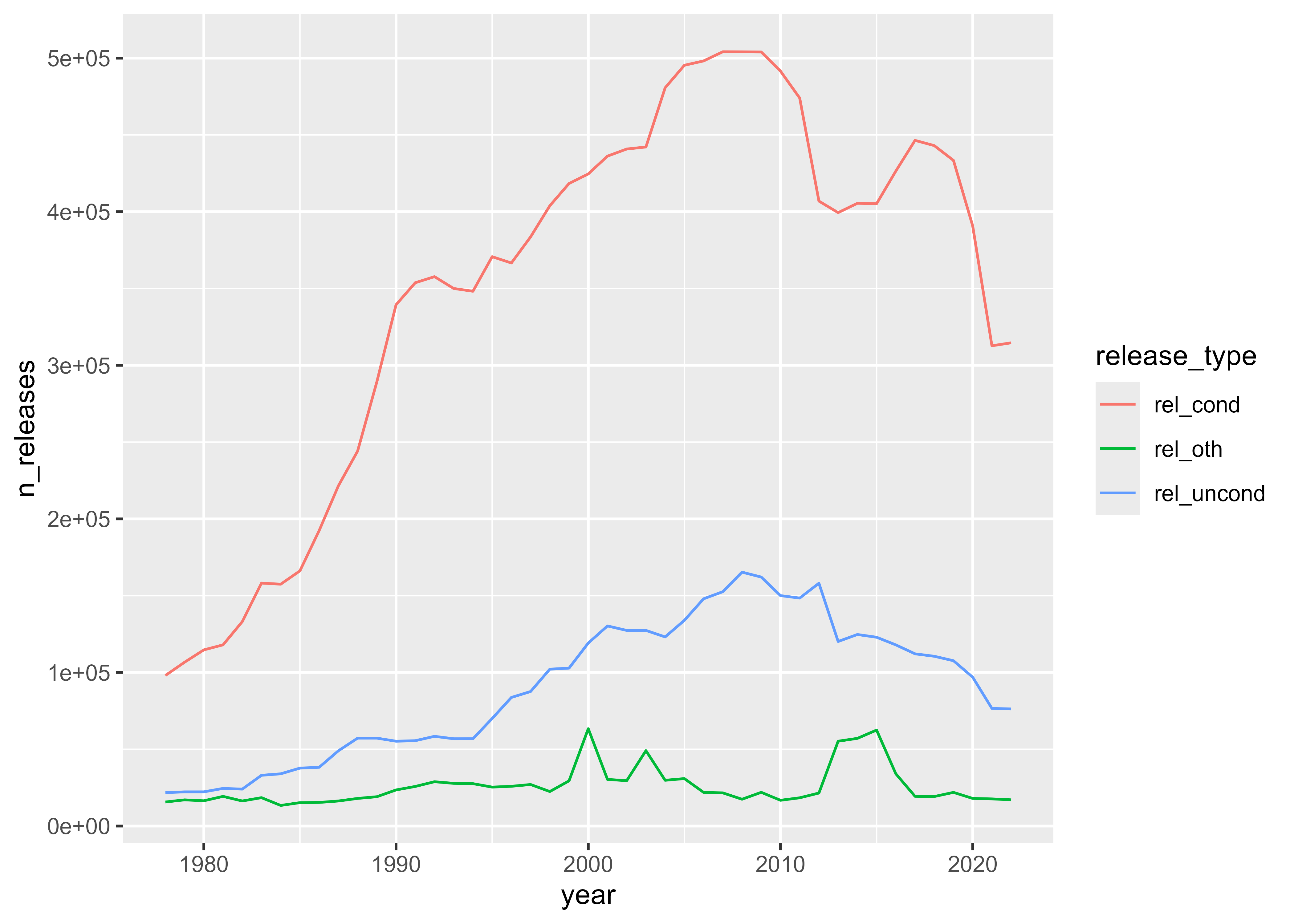
releases_us |>
  ggplot(aes(year, pct_releases, fill = release_type)) +
  geom_col()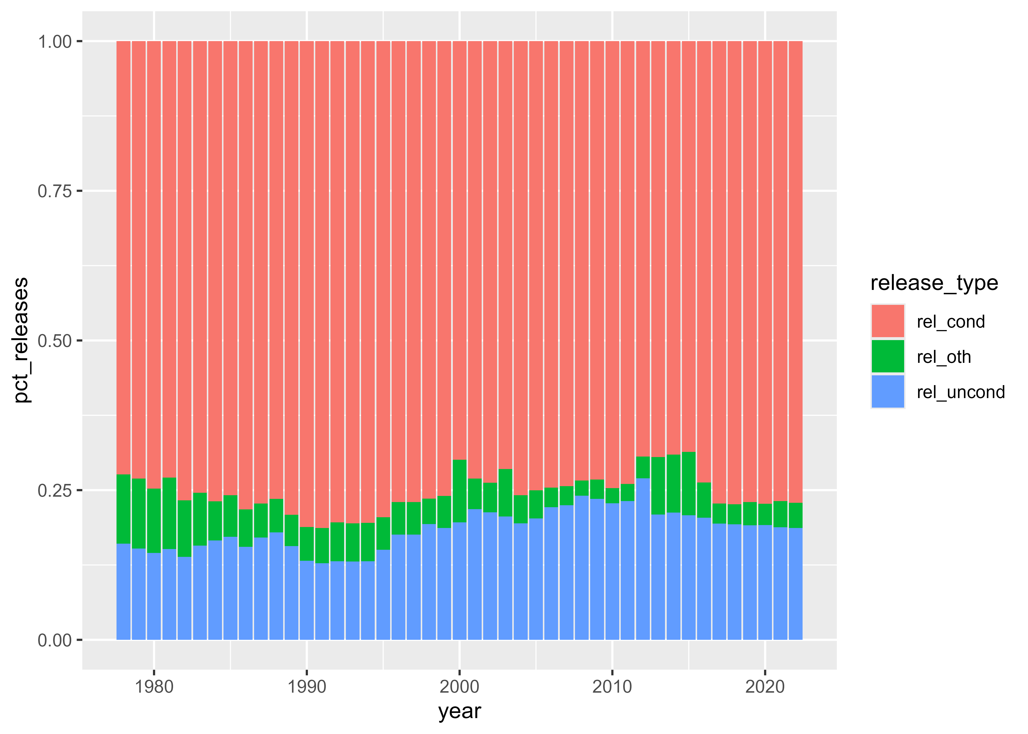
These plots show that the total number of people released from prison grew to a peak around 2010 and then declined. The share of people released with conditions has been fairly steady, while the share of people released without conditions has increased slightly since the late 1970s.
Long to wide
Most often, data needs to be reshaped from wide to long. But if you want to make long data wide, you can use the pivot_wider() function. Instead of specifying which columns to make long, you specify which column contains the names to use for the new columns and which column contains the values to place in those new columns. Starting with the tidied dataset, you can use pivot_wider() to return this data frame to its original, wide format.
nps_release_tidy |>
  pivot_wider(names_from = release_type, values_from = n_releases)
# A tibble: 4,590 × 7
year state_name state_abbr sex rel_uncond rel_cond rel_oth
<dbl> <chr> <chr> <chr> <dbl> <dbl> <dbl>
1 1978 Alabama AL m 1070 1485 252
2 1978 Alabama AL f 46 92 20
3 1979 Alabama AL m 723 1777 272
4 1979 Alabama AL f 33 174 8
5 1980 Alabama AL m 524 2173 552
6 1980 Alabama AL f 24 147 16
7 1981 Alabama AL m 520 1695 746
8 1981 Alabama AL f 20 137 63
9 1982 Alabama AL m 1097 1451 349
10 1982 Alabama AL f 44 118 10
# ℹ 4,580 more rowsTidying data can be more of an art than a science; depending on your analytic needs, exactly what constitutes a tidy data set may differ. One sign that you may need to tidy your data is if you’re unable to use the core tidyverse functions for data analysis and plotting with the structure of your data. Recognizing untidy data and tidying it is a skill that takes experience and something that you will develop as you continue to work with R.
Resources
- R for Data Science (2e), Chapter 5 Data tidying: https://r4ds.hadley.nz/data-tidy
- tidyr Pivoting vignette: https://tidyr.tidyverse.org/articles/pivot.html
- Tidy Data, Journal of Statistical Software, 59(10), 1–23: https://www.jstatsoft.org/article/view/v059i10