library(tidyverse)
library(readxl)

nps_admit <- read_csv("data/nps-admissions.csv")
nps_release <- read_excel("data/nps-releases.xlsx")Lesson 14: Join Data
Introduction
The prior lessons focused on data analysis and manipulation with one dataset at a time. But in most real data analysis projects, you will have multiple datasets that contain different segments of data. This is especially true for data that is sourced from relational databases. Think about all the tables that are part of the data system that tracks people who are incarcerated. There are likely tables relating to individual characteristics like date of birth and gender, tables containing risk score or other evaluation data, tables with information about facility movements, and more. This is also the case for data stored across multiple Excel sheets or workbooks. To analyze this kind of data, you need to combine or join multiple tables to create a useful analytic dataset.
This lesson will introduce joins and demonstrate how to merge two tables with common variables or keys. Joining data is a complex topic and this lesson won’t cover everything, but it will show you the basics of how to combine data frames in R. Joins are a very common technique in querying relational databases, and many of the R functions described in this lesson are inspired by SQL’s join syntax. If you have experience writing SQL queries, the concepts in this lesson will be familiar to you.
The Joins chapter of R for Data Science offers a more in-depth discussion of joins.
For this lesson, you’ll need both the NPS admissions file and the NPS releases file. Read them in to R with the following code:
Keys
An important concept when thinking about joining tables is keys. There are different kinds of keys (primary, foreign, compound, etc.), but the core principle is that there must be some shared element between tables that allows you to connect the two tables. Often, this is a common column or variable such as an ID number, in the case of individual data. Generally, keys are a column or set of columns that uniquely identify an observation.
Data prep
It makes it much easier to join data frames if your data is in a tidy format first. So before attempting any joins, clean up and filter the admissions and releases data.
First, filter the admissions dataset so that it only contains rows for total admissions from California. Next, create a total admissions column by adding male and female admissions. Lastly, keep only the year, state name, and total admissions columns.
ca_admissions <- nps_admit |>
  filter(adm_type == "adm_total", state_abbr == "CA") |>
  mutate(n_admissions = m + f) |>
  select(year, state_name, n_admissions)

ca_admissions
# A tibble: 45 × 3
year state_name n_admissions
<dbl> <chr> <dbl>
1 1978 California 12419
2 1979 California 15940
3 1980 California 14487
4 1981 California 18024
5 1982 California 22321
6 1983 California 27511
7 1984 California 29681
8 1985 California 37883
9 1986 California 48925
10 1987 California 59698
# ℹ 35 more rowsTo clean up the releases data, again filter it so that it only contains California data, then group by year and sum the total release column to get the number of releases for men and women combined.
ca_releases <- nps_release |>
  filter(state_abbr == "CA") |>
  group_by(year) |>
  summarize(n_releases = sum(rel_total)) |>
  ungroup()

ca_releases
# A tibble: 45 × 2
year n_releases
<dbl> <dbl>
1 1978 10207
2 1979 14230
3 1980 12483
4 1981 13375
5 1982 16651
6 1983 23069
7 1984 25923
8 1985 31256
9 1986 39526
10 1987 52611
# ℹ 35 more rowsSingle key join
Now you’re ready to join these two data frames to create a single data frame with both the number of admissions and the number of releases. To do this, start with the ca_admissions, then use the left_join function to join with the ca_releases dataset, specifying that the column (or key) to use to join is year. Specifying this key ensures that the row with the number of admissions from 1978 is combined with the row with the number of releases from 1978, and so on for each year.
ca_admissions |>
  left_join(ca_releases, join_by("year"))
# A tibble: 45 × 4
year state_name n_admissions n_releases
<dbl> <chr> <dbl> <dbl>
1 1978 California 12419 10207
2 1979 California 15940 14230
3 1980 California 14487 12483
4 1981 California 18024 13375
5 1982 California 22321 16651
6 1983 California 27511 23069
7 1984 California 29681 25923
8 1985 California 37883 31256
9 1986 California 48925 39526
10 1987 California 59698 52611
# ℹ 35 more rowsMultiple key join
This worked well for the California data, but what if you wanted to join the admissions and releases datasets for all states? Let’s try it! First, perform some data wrangling to tidy these data frames.
all_admissions <- nps_admit |>
  filter(adm_type == "adm_total") |>
  mutate(n_admissions = m + f) |>
  select(year, state_name, n_admissions)

all_admissions
# A tibble: 2,295 × 3
year state_name n_admissions
<dbl> <chr> <dbl>
1 1978 Alabama 2815
2 1979 Alabama 2819
3 1980 Alabama 3774
4 1981 Alabama 4025
5 1982 Alabama 4473
6 1983 Alabama 4662
7 1984 Alabama 4755
8 1985 Alabama 4407
9 1986 Alabama 4284
10 1987 Alabama 4843
# ℹ 2,285 more rowsall_releases <- nps_release |>
group_by(year, state_name) |>
summarize(n_releases = sum(rel_total)) |>
ungroup()
all_releases# A tibble: 2,295 × 3
year state_name n_releases
<dbl> <chr> <dbl>
1 1978 Alabama 2984
2 1978 Alaska 322
3 1978 Arizona 1687
4 1978 Arkansas 1908
5 1978 California 10207
6 1978 Colorado 1372
7 1978 Connecticut 1716
8 1978 Delaware 508
9 1978 District of Columbia 3335
10 1978 Florida 7741
# ℹ 2,285 more rowsNext, join admissions and releases by year.
all_admissions |>
  left_join(all_releases, join_by("year"))
Warning in left_join(all_admissions, all_releases, join_by("year")): Detected an unexpected many-to-many relationship between `x` and `y`.
ℹ Row 1 of `x` matches multiple rows in `y`.
ℹ Row 1 of `y` matches multiple rows in `x`.
ℹ If a many-to-many relationship is expected, set `relationship =
"many-to-many"` to silence this warning.# A tibble: 117,045 × 5
year state_name.x n_admissions state_name.y n_releases
<dbl> <chr> <dbl> <chr> <dbl>
1 1978 Alabama 2815 Alabama 2984
2 1978 Alabama 2815 Alaska 322
3 1978 Alabama 2815 Arizona 1687
4 1978 Alabama 2815 Arkansas 1908
5 1978 Alabama 2815 California 10207
6 1978 Alabama 2815 Colorado 1372
7 1978 Alabama 2815 Connecticut 1716
8 1978 Alabama 2815 Delaware 508
9 1978 Alabama 2815 District of Columbia 3335
10 1978 Alabama 2815 Florida 7741
# ℹ 117,035 more rowsOops! What just happened there? Look at the warning message that indicates that there are multiple row matches between the two tables. Next, notice the number of rows in the joined dataset: 117,045! That’s a lot more than the 2,295 rows in the admissions and releases data frames. Finally, see that there are 2 state name columns in the joined data frame (state_name.x and state_name.y). All of this points to an issue with the join that is important to examine.
The problem is that the code above only specifies the year column as the join. So, every 1978 row in the admissions data was matched to every 1978 row in the releases data. Look at the second row in the joined data above: the number of admissions in Alabama in 1978 is in the same row as the number of releases in Alaska in 1978.
To fix this problem, the join needs to be made on two columns: year and state_name. This ensures that rows from each table match both the year and state as they are combined.
all_admissions |>
  left_join(all_releases, join_by("year", "state_name"))
# A tibble: 2,295 × 4
year state_name n_admissions n_releases
<dbl> <chr> <dbl> <dbl>
1 1978 Alabama 2815 2984
2 1979 Alabama 2819 3005
3 1980 Alabama 3774 3452
4 1981 Alabama 4025 3194
5 1982 Alabama 4473 3091
6 1983 Alabama 4662 3602
7 1984 Alabama 4755 4150
8 1985 Alabama 4407 3904
9 1986 Alabama 4284 3529
10 1987 Alabama 4843 3745
# ℹ 2,285 more rowsNow, there is no warning about multiple matches, the resulting data frame has the same number of rows as the admissions and releases data frames, and there are no extra columns. This join was successful!
Types of joins
In the examples above, there were the same number of rows in each of the datasets to be joined, and each row in nps_admit matched to a single row in nps_release. But this isn’t always the case with real-life data. Consider trying to join the all_releases data frame with the ca_admissions data frame:
all_releases |>
  left_join(ca_admissions, join_by("year", "state_name"))
# A tibble: 2,295 × 4
year state_name n_releases n_admissions
<dbl> <chr> <dbl> <dbl>
1 1978 Alabama 2984 NA
2 1978 Alaska 322 NA
3 1978 Arizona 1687 NA
4 1978 Arkansas 1908 NA
5 1978 California 10207 12419
6 1978 Colorado 1372 NA
7 1978 Connecticut 1716 NA
8 1978 Delaware 508 NA
9 1978 District of Columbia 3335 NA
10 1978 Florida 7741 NA
# ℹ 2,285 more rowsNotice that there are rows with missing or NA values in the n_admissions column. In fact, the only rows with non-missing data are California rows. This makes sense, because the admissions data used in the join is the filtered ca_admissions dataset.
To understand why this is happening and how to adjust your code to handle joining data frames with different numbers of observations, the next sections discuss different types of joins.
Left join
In a left join, all the rows in the first (or left) data frame are retained, and the rows in the second (or right) data frame that match the first data frame are joined. If there are rows in the first data frame with no match in the second data frame, NA or missing values will be added in the joined columns. Additionally, if there are rows in the second data frame that don’t match to a key in the first data frame, they are not included in the joined data frame.
This animation shows a left join:

Inner join
In an inner join, only rows where there are matching columns in both the first and second data frame are retained. If there are rows in the first data frame with no match in the second data frame, they are discarded. Similarly, if there are rows in the second data frame with no match in the first data frame, they are also discarded.
This animation shows an inner join:
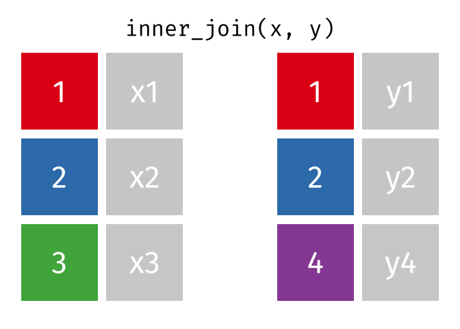
To perform an inner join in R, use the same code as above, but replace left_join with inner_join. In this case, the resulting joined data frame only has rows for California, even though the first data frame (all_releases) has rows for all states. Because the second data frame (ca_admissions) only has California rows, all non-matching rows from the first data frame are dropped.
all_releases |>
  inner_join(ca_admissions, join_by("year", "state_name"))
# A tibble: 45 × 4
year state_name n_releases n_admissions
<dbl> <chr> <dbl> <dbl>
1 1978 California 10207 12419
2 1979 California 14230 15940
3 1980 California 12483 14487
4 1981 California 13375 18024
5 1982 California 16651 22321
6 1983 California 23069 27511
7 1984 California 25923 29681
8 1985 California 31256 37883
9 1986 California 39526 48925
10 1987 California 52611 59698
# ℹ 35 more rowsFull join
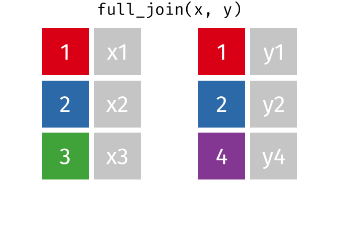
A full join keeps all rows and all columns from both the first and second data frames, regardless of matching. In rows where there are no matching values, NA is returned, similar to a left join.
This animation shows a full join:
Why join?
Often, to do any useful analysis, you’ll need to join multiple data frames. By looking at admissions and releases separately in prior lessons in this course, you missed out on some interesting trends. Now that you’re able to join data, one way to show these population movements would be to plot admissions and releases on the same chart.
To make this plot, start by joining California admissions and releases and then pivot the data frame so that admissions and releases become rows instead of columns.
ca_adm_rel_tidy <- ca_admissions |>
  left_join(ca_releases, join_by("year")) |>
  pivot_longer(starts_with("n"), names_to = "movement", values_to = "n")
From there, make a dodged bar chart with year on the x-axis, n on the y-axis, and the type of movement (admissions or release) as the fill. To make a chart where the bars are next to one another (rather than stacked) use position_dodge().
ca_adm_rel_tidy |>
  ggplot(aes(x = year, y = n, fill = movement)) +
  geom_col(position = position_dodge()) +
  scale_fill_manual(
    values = c("coral", "steelblue"),
    labels = c("Admissions", "Releases")
    ) +
  scale_y_continuous(labels = scales::label_comma()) +
  labs(
    title = "California Prison Admissions and Releases",
    caption = "BJS National Prisoner Statistics",
    x = NULL,
    y = NULL,
    fill = NULL
    ) +
  theme_minimal()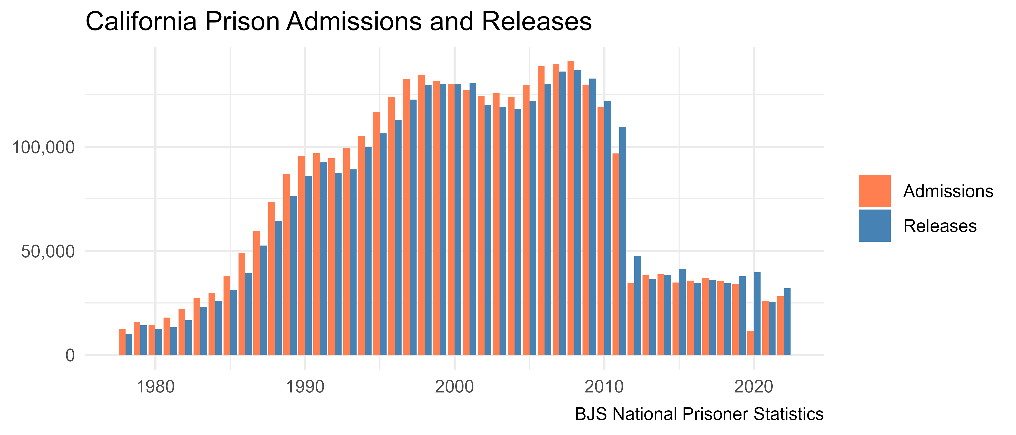
In California, more people were admitted than released from 1978 through the mid 2000s. Starting in 2008, more people were released than admitted in most years, and there was a huge drop in both admissions and releases starting in 2012. A big driver of this change was the prison realignment reform, which shifted responsibility from the state to the county for people convicted of low-level offenses.
The response to the COVID-19 pandemic is also apparent from this chart, where in 2020 far more people were released from prison in California than were admitted.
Resources
- R for Data Science (2e), Chapter 19 Joins: https://r4ds.hadley.nz/joins.html
- dplyr Two-table verbs vignette: https://dplyr.tidyverse.org/articles/two-table.html