library(tidyverse)

arrests_file_url <- "https://github.com/CSGJusticeCenter/va_data/raw/refs/heads/main/courses/intro_r/arrests.csv"
arrests <- read_csv(arrests_file_url)Lesson 16: Dates and Times
Introduction
The data that you’ve worked with in this course so far has been either numbers or text. This lesson focuses on two special kinds of numeric data: dates and times. While dates and times appear relatively straightforward, there are all sorts of complexities that must be considered when programming or doing math with dates and times. For example, how many days are in a month? Or a year? How about time zones and daylight-saving time? This lesson won’t get into all these topics, but it’s important to be aware of the many possible edge cases that can impact date and time data.
Most of the functions that you’ll use in this lesson come from the lubridate R package. You don’t need to separately install or attach lubridate because it is part of the tidyverse.
Chapter 17 of R for Data Science discusses more of these complexities.
The NPS data that you’ve been working with in this course so far doesn’t have dates and times, so for this lesson, you’ll use arrest data. This is a modified and simplified version of data about arrests released publicly by a police department. Instead of saving this data locally and reading it in as you’ve done with the NPS data, read this data directly into your R session from a CSV file saved on the web.
This is a convenience feature of read_csv() that allows you to provide the URL of the CSV file, and read_csv() will download that file to a temporary location on your computer, read it in to R, and then delete the temp file. This can be especially useful with a file that changes frequently, so that you can read in the most recent version rather than manually downloading and saving the file from the web.
Now that you have the arrests data in your R session, do some quick exploration.
arrests# A tibble: 1,000 × 9
arrest_id arrest_date arrest_time booking_year booking_month booking_day
<dbl> <chr> <chr> <dbl> <chr> <dbl>
1 1 2/4/2020 14 10 2020 February 4
2 2 6/28/2022 20 30 2022 June 28
3 3 5/1/2023 10 00 2023 May 1
4 4 10/19/2021 17 00 2021 October 19
5 5 11/30/2021 00 30 2021 November 30
6 6 1/8/2022 20 30 2022 January 8
7 7 5/28/2022 22 00 2022 May 29
8 8 4/27/2021 03 15 2021 April 27
9 9 1/14/2020 23 50 2020 January 15
10 10 3/29/2021 00 47 2021 March 29
# ℹ 990 more rows
# ℹ 3 more variables: booking_time <chr>, arrest_type <chr>, charge_group <chr>How many rows and columns are there? What data types are those columns stored as? How many arrest types are there?
arrests |>
  count(arrest_type)
# A tibble: 3 × 2
arrest_type n
<chr> <int>
1 F 624
2 I 1
3 M 375What are the most frequent charge groups?
arrests |>
  count(charge_group, sort = TRUE)
# A tibble: 22 × 2
charge_group n
<chr> <int>
1 Aggravated Assault 175
2 Miscellaneous Other Violations 152
3 Other Assaults 116
4 Narcotic Drug Laws 85
5 Driving Under Influence 83
6 Weapon (carry/poss) 77
7 Vehicle Theft 75
8 Larceny 45
9 Robbery 39
10 Burglary 33
# ℹ 12 more rowsDates
You might have noticed that the arrest_date column is stored as a character or string variable (chr). While it looks like a date in the data preview, it doesn’t act like a date. Try to sort by the arrest date column to see what’s going on:
arrests |>
  arrange(arrest_date)
# A tibble: 1,000 × 9
arrest_id arrest_date arrest_time booking_year booking_month booking_day
<dbl> <chr> <chr> <dbl> <chr> <dbl>
1 891 1/1/2022 03 55 2022 January 1
2 166 1/1/2023 02 45 2023 January 1
3 403 1/1/2024 01 30 2024 January 1
4 83 1/10/2020 11 45 2020 January 10
5 800 1/10/2022 08 00 2022 January 10
6 770 1/11/2020 19 30 2020 January 11
7 797 1/11/2020 23 40 2020 January 12
8 293 1/11/2021 07 30 2021 January 11
9 377 1/13/2021 17 00 2021 January 13
10 315 1/13/2022 11 22 2022 January 13
# ℹ 990 more rows
# ℹ 3 more variables: booking_time <chr>, arrest_type <chr>, charge_group <chr>If this column sorted correctly as a date, all the 2020 arrests would be before any arrests in 2021 or later. To get these dates to act like dates, you need to convert the arrest_date column from a character variable into a date variable. Use the mdy() function to convert the character to a date and specify that the data in the arrest_date column is stored in the month/day/year.
arrests |>
  mutate(arrest_date = mdy(arrest_date)) |>
  arrange(arrest_date)
# A tibble: 1,000 × 9
arrest_id arrest_date arrest_time booking_year booking_month booking_day
<dbl> <date> <chr> <dbl> <chr> <dbl>
1 366 2020-01-02 11 45 2020 January 2
2 647 2020-01-03 07 40 2020 January 3
3 239 2020-01-04 22 40 2020 January 5
4 586 2020-01-04 01 10 2020 January 4
5 717 2020-01-04 18 00 2020 January 4
6 990 2020-01-04 14 45 2020 January 4
7 878 2020-01-05 09 00 2020 January 5
8 116 2020-01-06 22 10 2020 January 7
9 820 2020-01-08 13 45 2020 January 8
10 978 2020-01-08 02 00 2020 January 8
# ℹ 990 more rows
# ℹ 3 more variables: booking_time <chr>, arrest_type <chr>, charge_group <chr>Now, you can see arrest_date is a date column type and the data frame is now sorted in correct chronological order.
Dates from multiple columns
For the booking date, there are three separate columns: booking_year, booking_month, and booking_day. Year and day are numbers, and the month is written out in text. To create a booking_date column from these three columns, you can use a process similar to how you made arrest_date with a couple of small additions. First, use the paste() function to combine booking_year, booking_month, and booking_day into a single string and then use ymd() to create the date. Use ymd() (year, month, day) instead of mdy() (month, day, year) because in this case, the year comes first in the character you’re converting to a date.
arrests |>
  mutate(booking_date = ymd(paste(booking_year, booking_month, booking_day))) |>
  select(starts_with("booking"))
# A tibble: 1,000 × 5
booking_year booking_month booking_day booking_time booking_date
<dbl> <chr> <dbl> <chr> <date>
1 2020 February 4 16 44 2020-02-04
2 2022 June 28 22 36 2022-06-28
3 2023 May 1 10 39 2023-05-01
4 2021 October 19 21 27 2021-10-19
5 2021 November 30 02 37 2021-11-30
6 2022 January 8 22 16 2022-01-08
7 2022 May 29 09 47 2022-05-29
8 2021 April 27 06 10 2021-04-27
9 2020 January 15 00 53 2020-01-15
10 2021 March 29 04 48 2021-03-29
# ℹ 990 more rowsGenerally, mdy(), ymd(), and dmy() are pretty good at parsing whatever input you throw at them. But if you’re having trouble converting text to dates with these functions, you may need to adjust or manipulate the input string.
Create a new data frame with arrest and booking dates converted to date columns and remove the booking year, month, and day columns.
arrests_date_clean <- arrests |>
  mutate(
    arrest_date = mdy(arrest_date),
    booking_date = ymd(paste(booking_year, booking_month, booking_day))
    ) |>
  select(-c(booking_year, booking_month, booking_day))
Extract components of dates
One useful thing you can do with a date column is extract components from the date. For instance, if you want to create new arrest_year and arrest_month columns, you can do that with the year() and month() functions.
arrests_date_clean |>
  mutate(
    arrest_year = year(arrest_date),
    arrest_month = month(arrest_date)
    ) |>
  select(starts_with("arrest"))
# A tibble: 1,000 × 6
arrest_id arrest_date arrest_time arrest_type arrest_year arrest_month
<dbl> <date> <chr> <chr> <dbl> <dbl>
1 1 2020-02-04 14 10 F 2020 2
2 2 2022-06-28 20 30 M 2022 6
3 3 2023-05-01 10 00 M 2023 5
4 4 2021-10-19 17 00 F 2021 10
5 5 2021-11-30 00 30 F 2021 11
6 6 2022-01-08 20 30 F 2022 1
7 7 2022-05-28 22 00 F 2022 5
8 8 2021-04-27 03 15 F 2021 4
9 9 2020-01-14 23 50 F 2020 1
10 10 2021-03-29 00 47 F 2021 3
# ℹ 990 more rowsYou can also extract the month as a name, rather than a number, by setting label = TRUE.
arrests_date_clean |>
  mutate(
    arrest_year = year(arrest_date),
    arrest_month = month(arrest_date, label = TRUE, abbr = FALSE)
    ) |>
  select(starts_with("arrest"))
# A tibble: 1,000 × 6
arrest_id arrest_date arrest_time arrest_type arrest_year arrest_month
<dbl> <date> <chr> <chr> <dbl> <ord>
1 1 2020-02-04 14 10 F 2020 February
2 2 2022-06-28 20 30 M 2022 June
3 3 2023-05-01 10 00 M 2023 May
4 4 2021-10-19 17 00 F 2021 October
5 5 2021-11-30 00 30 F 2021 November
6 6 2022-01-08 20 30 F 2022 January
7 7 2022-05-28 22 00 F 2022 May
8 8 2021-04-27 03 15 F 2021 April
9 9 2020-01-14 23 50 F 2020 January
10 10 2021-03-29 00 47 F 2021 March
# ℹ 990 more rowsDate-times
The arrest dataset also contains columns for arrest time and booking time. In addition to the date data type, R also can store date-times, and there are functions that help create date-times similar to the date helpers. In this case, the time column we have represents hours and minutes (no seconds), so you can use ymd_hm() (year, month, day, hour, minute) to create the date-time columns.
arrests_date_clean |>
  mutate(
    arrest_date_time = ymd_hm(paste(arrest_date, arrest_time)),
    booking_date_time = ymd_hm(paste(booking_date, booking_time)),
    ) |>
  select(arrest_date, arrest_time, arrest_date_time,
         booking_date, booking_time, booking_date_time)
# A tibble: 1,000 × 6
arrest_date arrest_time arrest_date_time booking_date booking_time
<date> <chr> <dttm> <date> <chr>
1 2020-02-04 14 10 2020-02-04 14:10:00 2020-02-04 16 44
2 2022-06-28 20 30 2022-06-28 20:30:00 2022-06-28 22 36
3 2023-05-01 10 00 2023-05-01 10:00:00 2023-05-01 10 39
4 2021-10-19 17 00 2021-10-19 17:00:00 2021-10-19 21 27
5 2021-11-30 00 30 2021-11-30 00:30:00 2021-11-30 02 37
6 2022-01-08 20 30 2022-01-08 20:30:00 2022-01-08 22 16
7 2022-05-28 22 00 2022-05-28 22:00:00 2022-05-29 09 47
8 2021-04-27 03 15 2021-04-27 03:15:00 2021-04-27 06 10
9 2020-01-14 23 50 2020-01-14 23:50:00 2020-01-15 00 53
10 2021-03-29 00 47 2021-03-29 00:47:00 2021-03-29 04 48
# ℹ 990 more rows
# ℹ 1 more variable: booking_date_time <dttm>To make this work, use paste() again to combine the existing arrest_date and arrest_time columns and then convert that string to date-time with ymd_hm().
arrests_date_time_clean <- arrests_date_clean |>
  mutate(
    arrest_date_time = ymd_hm(paste(arrest_date, arrest_time)),
    booking_date_time = ymd_hm(paste(booking_date, booking_time))
    ) |>
  select(-c(arrest_time, booking_time))
Math with dates and times
Now that you have the dates and times in a structured format, you can use those columns to perform calculations. A common calculation is determining the number of days between two dates. Simple subtraction works to find the number of days from arrest to booking.
arrests_date_time_clean |>
  mutate(arrest_to_booking_day = booking_date - arrest_date) |>
  select(arrest_date, booking_date, arrest_to_booking_day)
# A tibble: 1,000 × 3
arrest_date booking_date arrest_to_booking_day
<date> <date> <drtn>
1 2020-02-04 2020-02-04 0 days
2 2022-06-28 2022-06-28 0 days
3 2023-05-01 2023-05-01 0 days
4 2021-10-19 2021-10-19 0 days
5 2021-11-30 2021-11-30 0 days
6 2022-01-08 2022-01-08 0 days
7 2022-05-28 2022-05-29 1 days
8 2021-04-27 2021-04-27 0 days
9 2020-01-14 2020-01-15 1 days
10 2021-03-29 2021-03-29 0 days
# ℹ 990 more rowsMost bookings take place on the same day as an arrest, so a more interesting calculation to make is the amount of time between arrest and booking. Subtract arrest_date_time from booking_date_time to calculate this.
arrests_date_time_clean |>
  mutate(arrest_to_booking_min = booking_date_time - arrest_date_time) |>
  select(arrest_date_time, booking_date_time, arrest_to_booking_min)
# A tibble: 1,000 × 3
arrest_date_time booking_date_time arrest_to_booking_min
<dttm> <dttm> <drtn>
1 2020-02-04 14:10:00 2020-02-04 16:44:00 154 mins
2 2022-06-28 20:30:00 2022-06-28 22:36:00 126 mins
3 2023-05-01 10:00:00 2023-05-01 10:39:00 39 mins
4 2021-10-19 17:00:00 2021-10-19 21:27:00 267 mins
5 2021-11-30 00:30:00 2021-11-30 02:37:00 127 mins
6 2022-01-08 20:30:00 2022-01-08 22:16:00 106 mins
7 2022-05-28 22:00:00 2022-05-29 09:47:00 707 mins
8 2021-04-27 03:15:00 2021-04-27 06:10:00 175 mins
9 2020-01-14 23:50:00 2020-01-15 00:53:00 63 mins
10 2021-03-29 00:47:00 2021-03-29 04:48:00 241 mins
# ℹ 990 more rowsThere seems to be more variation in the number of minutes between arrest and booking than there was in the number of days. Create a dataset with this new variable so that you can do some deeper exploration.
arrests_calc <- arrests_date_time_clean |>
  mutate(arrest_to_booking_min = booking_date_time - arrest_date_time)
As usual, the first thing to do is look at your data! A good way to visualize the time from arrest to booking is with a histogram, which will show the distribution of time in the dataset.
arrests_calc |>
  ggplot(aes(arrest_to_booking_min)) +
  geom_histogram(binwidth = 15, color = "white")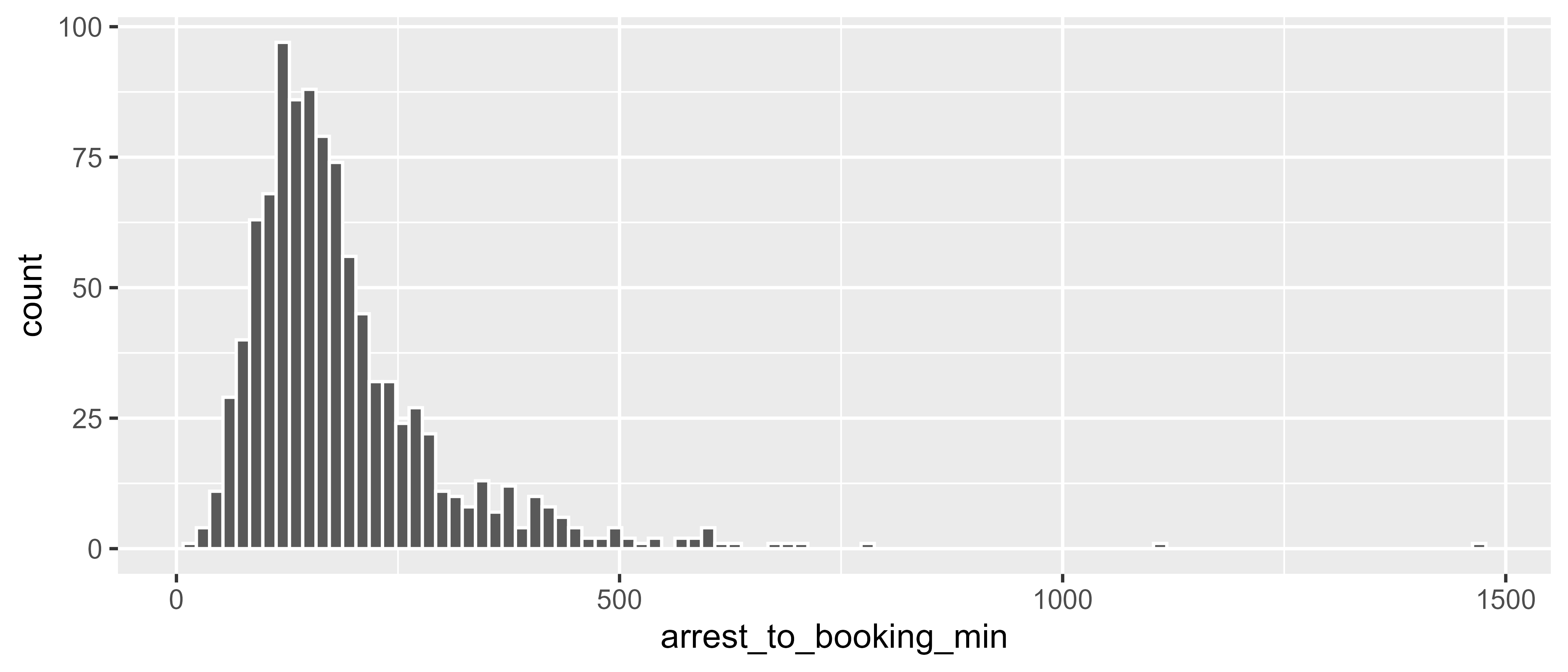
The distribution is skewed right, and the most common amount of time between arrest and booking is around three hours. But, it’s probably the case that there is more or less time between arrest and booking for certain types of arrests. There is an arrest_type column in the dataset, so you can use group_by() + summarize() to calculate the mean and median for each arrest type.
arrests_calc |>
  group_by(arrest_type) |>
  summarize(
    mean = mean(arrest_to_booking_min),
    median = median(arrest_to_booking_min)
  )
# A tibble: 3 × 3
arrest_type mean median
<chr> <drtn> <drtn>
1 F 200.4808 mins 170 mins
2 I 129.0000 mins 129 mins
3 M 166.4533 mins 148 minsIt looks like on average, there is slightly more time between arrest and booking for felony arrests than for misdemeanors or infractions. Another factor that may impact time to booking is the offense type. Look at the same summary statistics, but this time group by charge_group. Also, arrange the summarized dataset by mean so that you can see the charges with the most time between arrest and booking.
arrests_calc |>
  group_by(charge_group) |>
  summarize(
    mean = mean(arrest_to_booking_min),
    median = median(arrest_to_booking_min),
    ) |>
  arrange(desc(mean))
# A tibble: 22 × 3
charge_group mean median
<chr> <drtn> <drtn>
1 Rape 364.1250 mins 347.5 mins
2 Homicide 335.1000 mins 349.0 mins
3 Receive Stolen Property 249.1250 mins 190.0 mins
4 Fraud/Embezzlement 212.8000 mins 194.0 mins
5 Aggravated Assault 205.1714 mins 170.0 mins
6 Weapon (carry/poss) 198.7013 mins 162.0 mins
7 Against Family/Child 198.5000 mins 164.0 mins
8 Narcotic Drug Laws 194.0471 mins 165.0 mins
9 Robbery 193.2308 mins 172.0 mins
10 Prostitution/Allied 188.4375 mins 162.5 mins
# ℹ 12 more rowsRape and homicide are the offenses with the most time to booking, which makes sense because these are likely the most complex cases and may require additional processing or casework.
Resources
- R for Data Science (2e), Chapter 17 Dates and times: https://r4ds.hadley.nz/datetimes
- lubridate R package website: https://lubridate.tidyverse.org/