This is the final lesson of Introduction to R for Corrections Analysts. If you’ve made it this far, you should have learned a solid base of skills and concepts that will help you analyze, visualize, and communicate about data using R. This knowledge will help bring a reproducible, code-based approach to data analysis that makes it easier to automate tasks and perform quality assurance checks. And hopefully, this is still early in your R journey—there is so much more to learn!
One of the best resources for learning R that has been referenced in nearly every lesson in this course is R for Data Science by Hadley Wickham, Mine Çetinkaya-Rundel, and Garrett Grolemund. In addition to referring to the materials for this course, R for Data Science should be one of your go-to sources when you’re learning more about using R.
This lesson is different from others in this course in that it presents an example of how you might use the many R skills you’ve learned to create an example report using Quarto. This includes importing, wrangling, reshaping, and visualizing data.
Consider your current workflow and process for building reports. For many, this may involve running SQL queries to extract data from a database; using Excel to clean, manipulate, and visualize the data; and writing a report in Word with charts and tables copy and pasted from Excel. Especially if you have to create a report like this at a regular cadence, using a tool like Quarto to automate the report generation process may save hours of manual labor and reduce the possibilities of errors. A future Advancing Data in Corrections Academy course will be dedicated to creating automated reports, but for now, look at the code, text, and plots below with an eye toward how this type of product and workflow could enhance your work.
By default, the code to generate this document is hidden, but above each plot there is an option to show the R code that generates the output. You can also view the entire Quarto source for this document by clicking Code > View Source in the upper-right corner of this page. The full source code also shows the text elements in the report that are created dynamically, using code.
Arrest Report
Show the code
library(tidyverse)library(reactable)library(scales)library(ggrepel)# read in arrest dataarrests <-read_csv("https://github.com/CSGJusticeCenter/va_data/raw/refs/heads/main/courses/intro_r/arrests.csv")# set years to filter datamin_year <-2020max_year <-2024# create cleaned up arrest dataset with arrest and booking date-timesarrests_clean <- arrests |>mutate(arrest_date =mdy(arrest_date),booking_date =ymd(paste(booking_year, booking_month, booking_day)), arrest_date_time =ymd_hm(paste(arrest_date, arrest_time)),booking_date_time =ymd_hm(paste(booking_date, booking_time)),arrest_to_booking_min = booking_date_time - arrest_date_time,arrest_year =year(arrest_date),arrest_month =month(arrest_date),arrest_month_chr =month(arrest_date, label =TRUE, abbr =FALSE),arrest_month_abbr =month(arrest_date, label =TRUE, abbr =TRUE), ) |>select(arrest_id, arrest_type, charge_group, arrest_to_booking_min, arrest_date_time, booking_date_time, arrest_year, arrest_month, arrest_month_chr,arrest_month_abbr) |>filter(between(arrest_year, min_year, max_year))# set ggplot2 theme for all plotstheme_set(theme_minimal(base_size =13, base_family ="Public Sans"))# arrests by type/severity (felony, misdemenaor, infraction)arrests_by_type <- arrests_clean |>count(arrest_type)arrests_by_charge <- arrests_clean |>count(charge_group) |>mutate(pct = n /sum(n))arrests_by_year <- arrests_clean |>count(arrest_year)
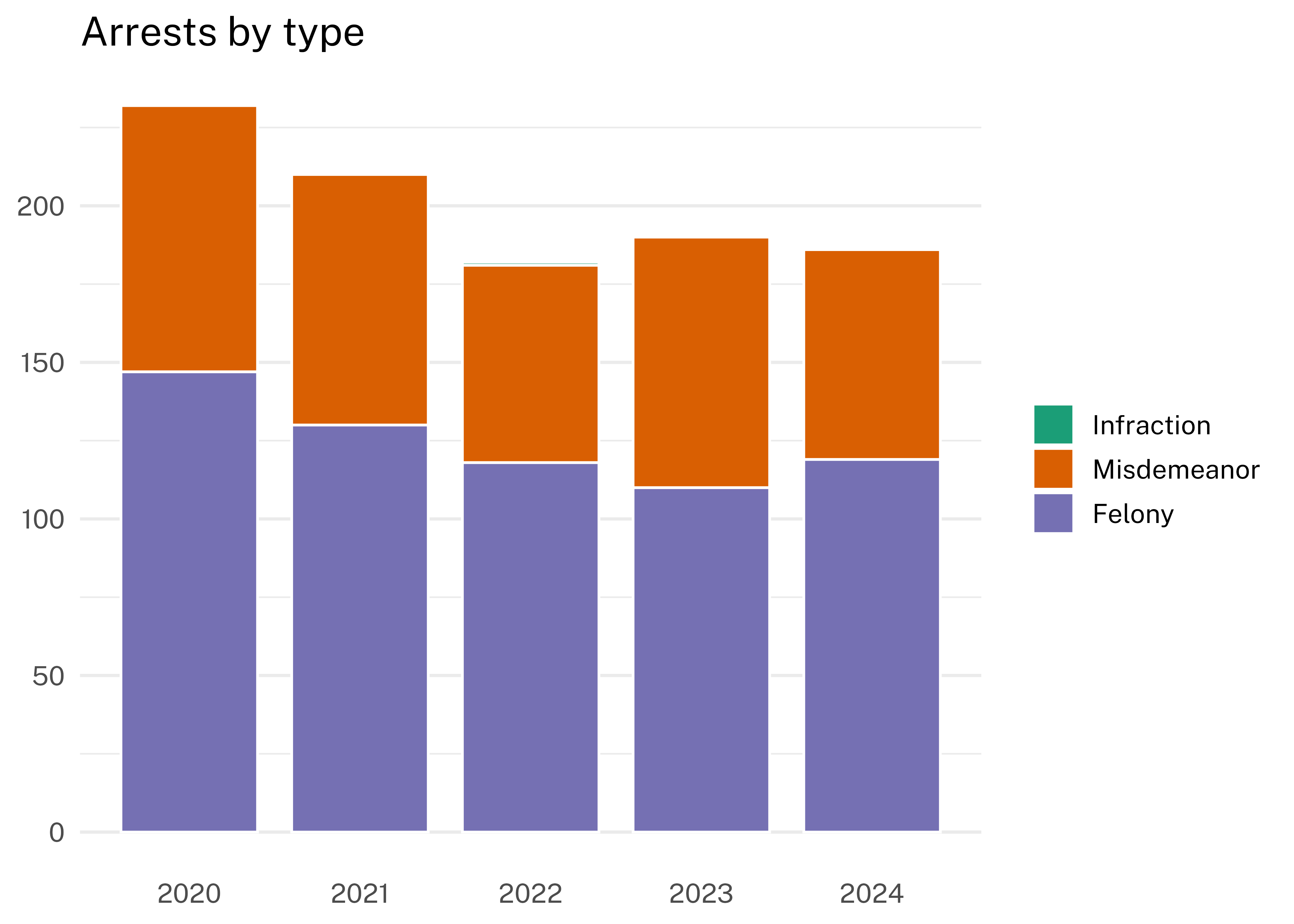
Since 2020, there have been 624 felony arrests, 375 misdemeanor arrests, and 1 infraction arrest. The year with the most arrests was 2020 in which there were 232 arrests. The year with the fewest arrests was 2022 in which there were 182 arrests.
The plot below shows the number of arrests by type for each year from 2020 to 2024.
arrests_by_charge <- arrests_clean |>count(charge_group) |>mutate(pct = n /sum(n)) |>arrange(desc(n))
The 3 most common charges over the 4 years were Aggravated Assault (175 arrests), Miscellaneous Other Violations (152 arrests), and Other Assaults (116 arrests).
The table below shows the number and percentage of arrests for each charge group.
Show the code
arrests_by_charge |>reactable(columns =list(charge_group =colDef(name ="Charge Group"),n =colDef(name ="# of Arrests"),pct =colDef(name ="% of Arrests",format =colFormat(percent =TRUE, digits =1)) ) )
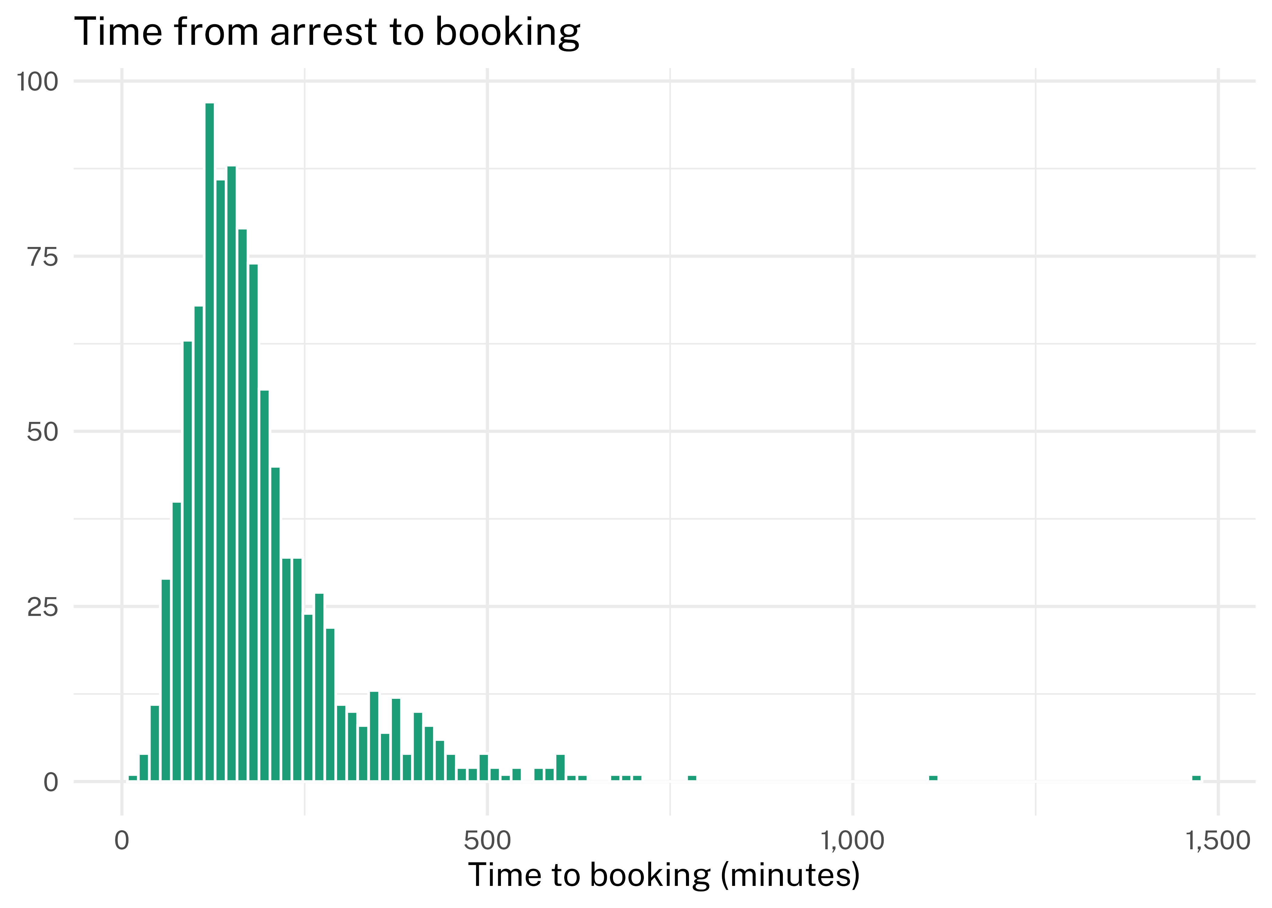
Over the 5-year period, the mean time from arrest to booking was 188 minutes, and the median time from arrest to booking was 160 minutes. The following histogram shows the distribution of time from arrest to booking. Each bar represents a 15-minute segment.
Show the code
arrests_clean |>ggplot(aes(arrest_to_booking_min)) +geom_histogram(binwidth =15, color ="white", fill =brewer_pal("qual", "Dark2")(1)) +scale_x_continuous(labels =label_comma()) +labs(title ="Time from arrest to booking",x ="Time to booking (minutes)",y =NULL )
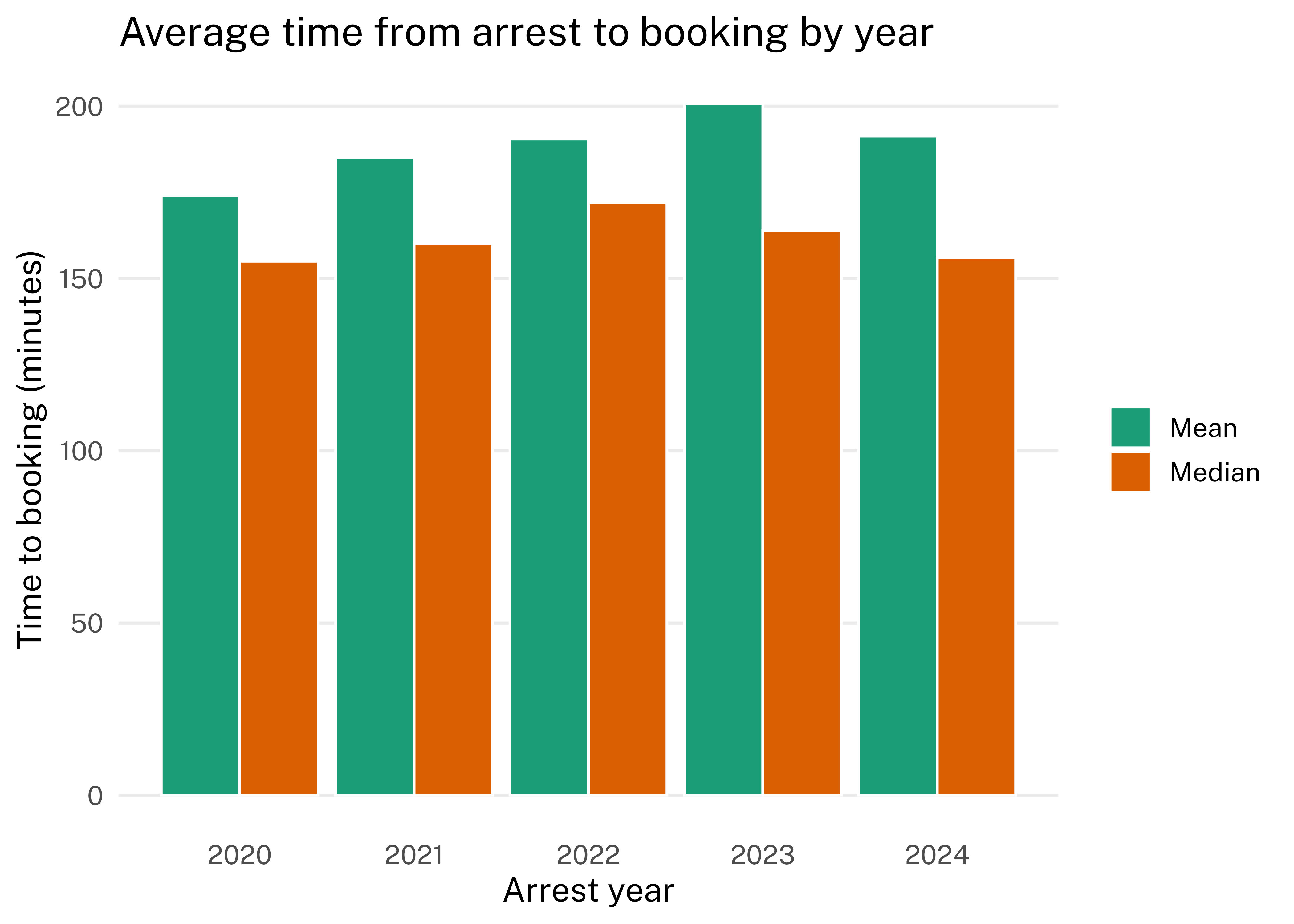
The time from arrest to booking also varied over time and by arrest type and charge group.
The year with the longest mean time to booking was 2023 (201 minutes) and the year with the shortest mean time to booking was 2020 (174 minutes).
Show the code
arrest_by_year_avg_pivot |>ggplot(aes(arrest_year, value, fill = name)) +geom_col(color ="white", position =position_dodge()) +scale_fill_brewer(palette ="Dark2") +labs(title ="Average time from arrest to booking by year",x ="Arrest year",y ="Time to booking (minutes)",fill =NULL ) +theme(panel.grid.major.x =element_blank(),panel.grid.minor =element_blank() )
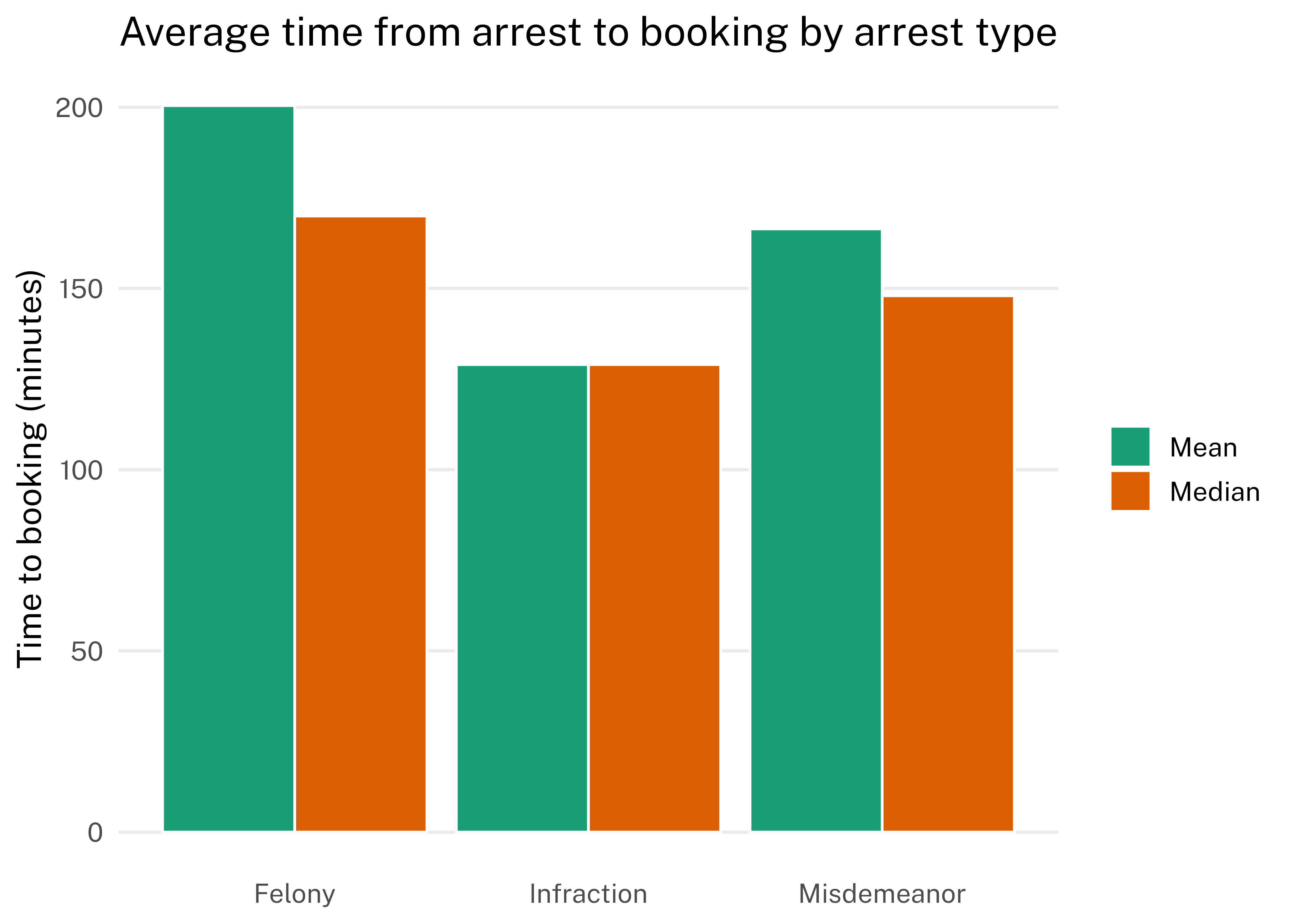
On average, the time from arrest to booking for felony arrests was 200 minutes, and the average time to booking for misdemeanor arrests was 166 minutes.
Show the code
arrest_by_type_avg_pivot |>ggplot(aes(arrest_type, value, fill = name)) +geom_col(color ="white", position =position_dodge()) +scale_fill_brewer(palette ="Dark2") +labs(title ="Average time from arrest to booking by arrest type",x =NULL,y ="Time to booking (minutes)",fill =NULL ) +theme(panel.grid.major.x =element_blank(),panel.grid.minor =element_blank() )
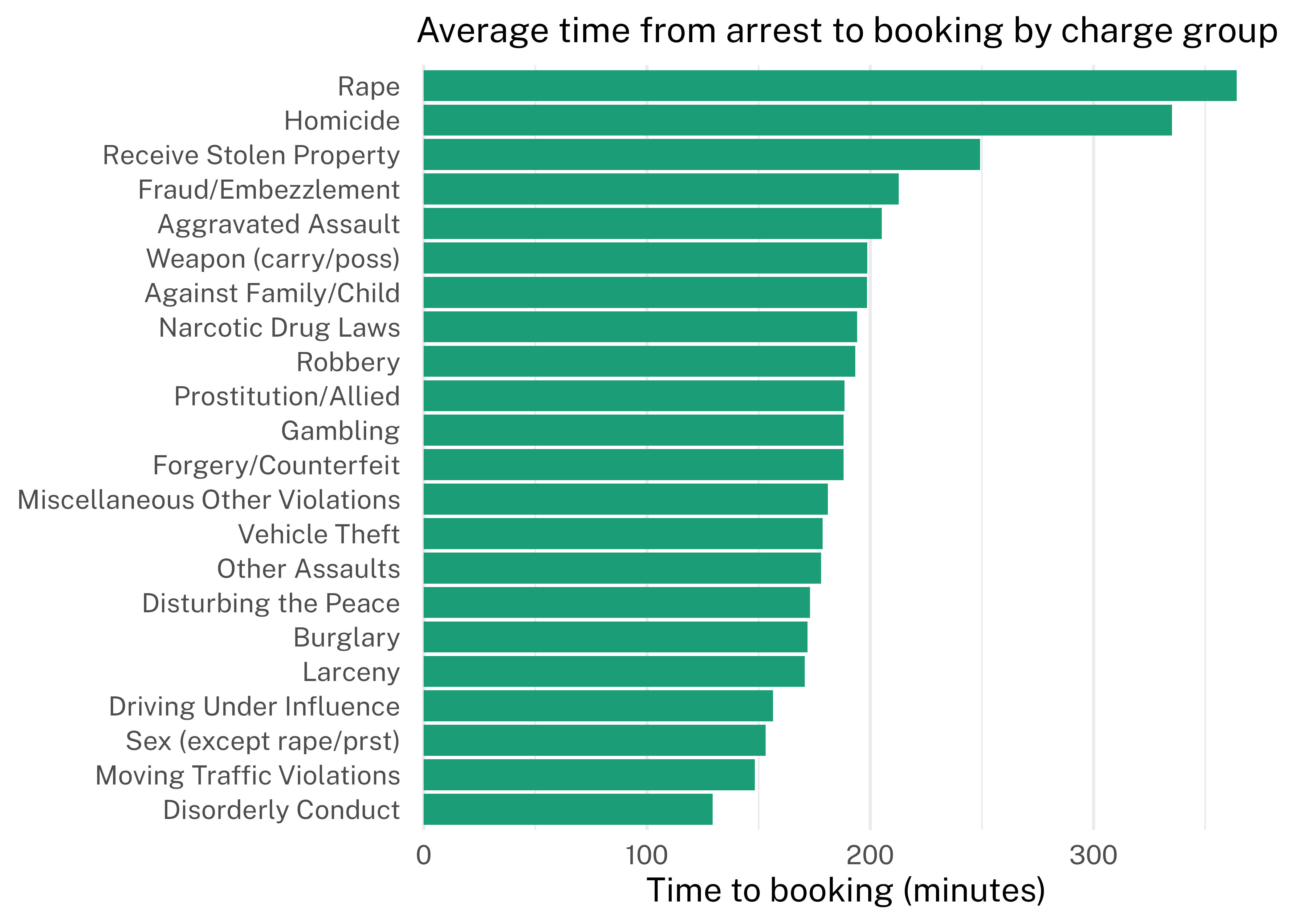
The charge with the longest mean time to booking was rape (364 minutes), and the charge with the shortest mean time to booking was disorderly conduct (129 minutes).
Show the code
time_to_booking_charge |>mutate(charge_group =fct_reorder(charge_group, mean)) |>ggplot(aes(mean, charge_group)) +geom_col(fill =brewer_pal("qual", "Dark2")(1)) +scale_x_continuous(expand =expansion(mult =c(0.01, 0.05))) +labs(title ="Average time from arrest to booking by charge group",x ="Time to booking (minutes)",y =NULL ) +theme(plot.title =element_text(size =13.7),panel.grid.major.y =element_blank(),panel.grid.minor.y =element_blank() )
This is the end of Introduction to R for Corrections Analysts, but hopefully not the end of you learning about R! Look for additional courses in the Advancing Data in Corrections Academy on more advanced R topics.
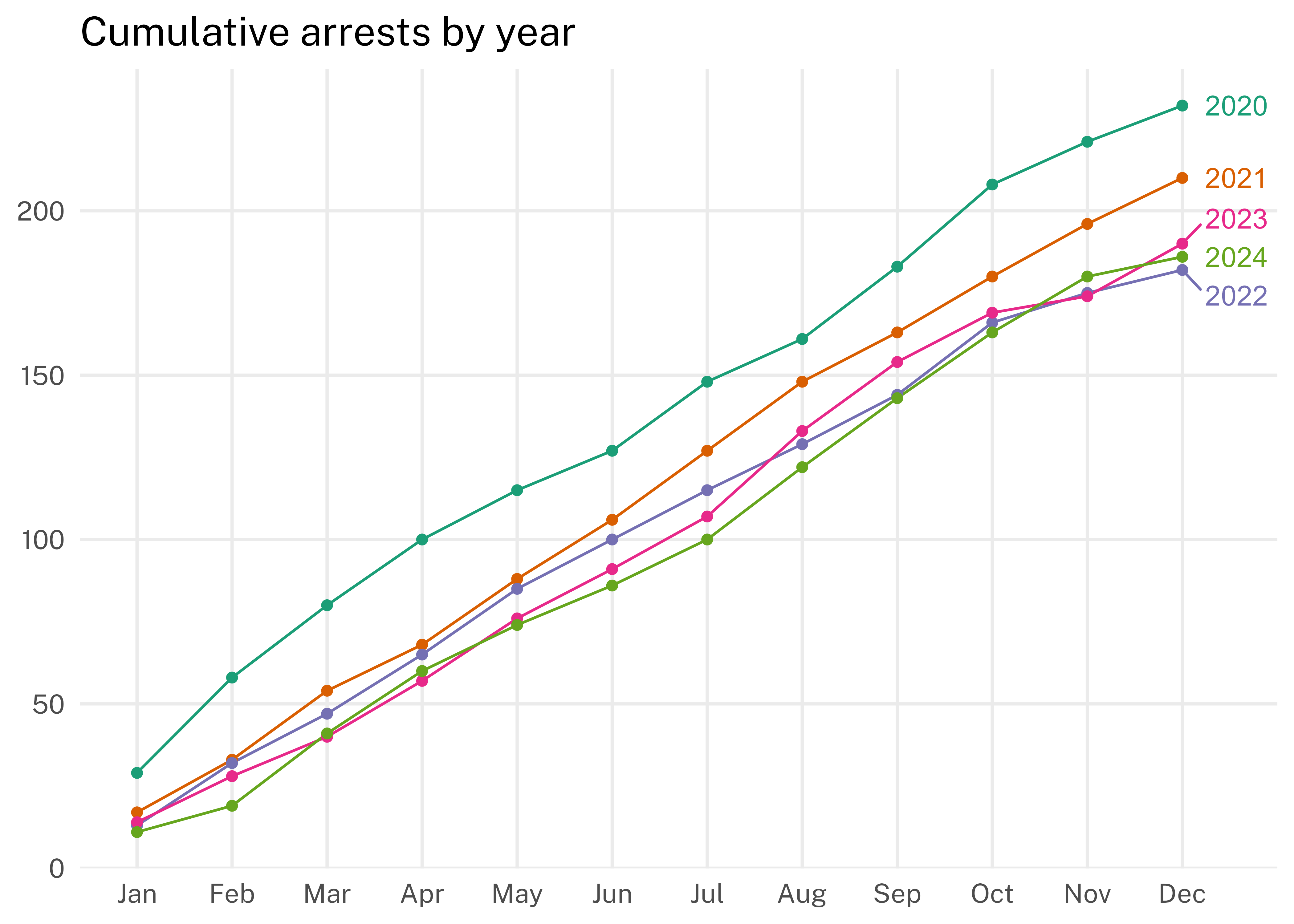
---title: "Lesson 22: Put It All Together"execute: warning: falseformat: html: code-fold: true code-summary: "Show the code" code-tools: true docx: code-fold: trueprefer-html: true---## IntroductionThis is the final lesson of Introduction to R for Corrections Analysts. If you've made it this far, you should have learned a solid base of skills and concepts that will help you analyze, visualize, and communicate about data using R. This knowledge will help bring a reproducible, code-based approach to data analysis that makes it easier to automate tasks and perform quality assurance checks. And hopefully, this is still early in your R journey---there is so much more to learn!One of the best resources for learning R that has been referenced in nearly every lesson in this course is [R for Data Science](https://r4ds.hadley.nz/) by Hadley Wickham, Mine Çetinkaya-Rundel, and Garrett Grolemund. In addition to referring to the materials for this course, R for Data Science should be one of your go-to sources when you're learning more about using R.This lesson is different from others in this course in that it presents an example of how you might use the many R skills you’ve learned to create an example report using Quarto. This includes importing, wrangling, reshaping, and visualizing data.Consider your current workflow and process for building reports. For many, this may involve running SQL queries to extract data from a database; using Excel to clean, manipulate, and visualize the data; and writing a report in Word with charts and tables copy and pasted from Excel. Especially if you have to create a report like this at a regular cadence, using a tool like Quarto to automate the report generation process may save hours of manual labor and reduce the possibilities of errors. A future Advancing Data in Corrections Academy course will be dedicated to creating automated reports, but for now, look at the code, text, and plots below with an eye toward how this type of product and workflow could enhance your work.By default, the code to generate this document is hidden, but above each plot there is an option to show the R code that generates the output. You can also view the entire Quarto source for this document by clicking Code > View Source in the upper-right corner of this page. The full source code also shows the text elements in the report that are created dynamically, using code.## Arrest Report```{r}library(tidyverse)library(reactable)library(scales)library(ggrepel)# read in arrest dataarrests <-read_csv("https://github.com/CSGJusticeCenter/va_data/raw/refs/heads/main/courses/intro_r/arrests.csv")# set years to filter datamin_year <-2020max_year <-2024# create cleaned up arrest dataset with arrest and booking date-timesarrests_clean <- arrests |>mutate(arrest_date =mdy(arrest_date),booking_date =ymd(paste(booking_year, booking_month, booking_day)), arrest_date_time =ymd_hm(paste(arrest_date, arrest_time)),booking_date_time =ymd_hm(paste(booking_date, booking_time)),arrest_to_booking_min = booking_date_time - arrest_date_time,arrest_year =year(arrest_date),arrest_month =month(arrest_date),arrest_month_chr =month(arrest_date, label =TRUE, abbr =FALSE),arrest_month_abbr =month(arrest_date, label =TRUE, abbr =TRUE), ) |>select(arrest_id, arrest_type, charge_group, arrest_to_booking_min, arrest_date_time, booking_date_time, arrest_year, arrest_month, arrest_month_chr,arrest_month_abbr) |>filter(between(arrest_year, min_year, max_year))# set ggplot2 theme for all plotstheme_set(theme_minimal(base_size =13, base_family ="Public Sans"))# arrests by type/severity (felony, misdemenaor, infraction)arrests_by_type <- arrests_clean |>count(arrest_type)arrests_by_charge <- arrests_clean |>count(charge_group) |>mutate(pct = n /sum(n))arrests_by_year <- arrests_clean |>count(arrest_year)```Since `{r} min_year`, there have been `{r} pull(filter(arrests_by_type, arrest_type == "F"), n)` felony arrests, `{r} pull(filter(arrests_by_type, arrest_type == "M"), n)` misdemeanor arrests, and `{r} pull(filter(arrests_by_type, arrest_type == "I"), n)` infraction arrest. The year with the most arrests was `{r} pull(filter(arrests_by_year, n == max(n)), arrest_year)` in which there were `{r} pull(filter(arrests_by_year, n == max(n)), n)` arrests. The year with the fewest arrests was `{r} pull(filter(arrests_by_year, n == min(n)), arrest_year)` in which there were `{r} pull(filter(arrests_by_year, n == min(n)), n)` arrests.The plot below shows the number of arrests by type for each year from `{r} min_year` to `{r} max_year`.```{r}arrests_clean |>count(year =year(arrest_date_time), arrest_type) |>mutate(arrest_type =fct_relevel(arrest_type, "I", "M", "F")) |>ggplot(aes(year, n, fill = arrest_type)) +geom_col(color ="white", width =0.8) +scale_fill_brewer(palette ="Dark2",labels =c("Infraction", "Misdemeanor", "Felony") ) +labs(title ="Arrests by type",x =NULL,y =NULL,fill =NULL ) +theme(panel.grid.major.x =element_blank(),panel.grid.minor.x =element_blank() )```### By month```{r}arrests_by_month <- arrests_clean |>count(arrest_month_chr) |>mutate(pct = n /sum(n))arrests_by_month_max <- arrests_by_month |>filter(n ==max(n))arrests_by_month_min <- arrests_by_month |>filter(n ==min(n))```Over the `{r} max_year - min_year` years of arrest data, `{r} percent(pull(arrests_by_month_max, pct), accuracy = 0.1, suffix = " percent")` of all arrests (`{r} pull(arrests_by_month_max, n)`) occurred in `{r} pull(arrests_by_month_max, arrest_month_chr)`, and `{r} percent(pull(arrests_by_month_min, pct), accuracy = 0.1, suffix = " percent")` of all arrests (`{r} pull(arrests_by_month_min, n)`) occurred in `{r} pull(arrests_by_month_min, arrest_month_chr)`.The plot below shows the cumulative number of arrests in each year by month.```{r}arrests_by_year_cum_sum <- arrests_clean |>count(arrest_year, arrest_month_abbr) |>group_by(arrest_year) |>mutate(arrests_cum =cumsum(n)) |>ungroup() |>mutate(arrest_year =as.character(arrest_year))arrests_by_year_cum_sum |>ggplot(aes( arrest_month_abbr, arrests_cum,color = arrest_year, group = arrest_year)) +geom_line() +geom_point() +geom_text_repel(data =filter(arrests_by_year_cum_sum, arrest_month_abbr =="Dec"),aes(label = arrest_year),nudge_x =1 ) +scale_color_brewer(palette ="Dark2") +labs(title ="Cumulative arrests by year",x =NULL,y =NULL ) +theme(legend.position ="none",panel.grid.minor =element_blank() )```### By charge```{r}arrests_by_charge <- arrests_clean |>count(charge_group) |>mutate(pct = n /sum(n)) |>arrange(desc(n))```The 3 most common charges over the `{r} max_year - min_year` years were `{r} arrests_by_charge[[1, 1]]` (`{r} arrests_by_charge[[1, 2]]` arrests), `{r} arrests_by_charge[[2, 1]]` (`{r} arrests_by_charge[[2, 2]]` arrests), and `{r} arrests_by_charge[[3, 1]]` (`{r} arrests_by_charge[[3, 2]]` arrests).The table below shows the number and percentage of arrests for each charge group.```{r}arrests_by_charge |>reactable(columns =list(charge_group =colDef(name ="Charge Group"),n =colDef(name ="# of Arrests"),pct =colDef(name ="% of Arrests",format =colFormat(percent =TRUE, digits =1)) ) )```### Time to booking```{r}time_to_booking_all <- arrests_clean |>summarize(n =n(),mean =as.numeric(mean(arrest_to_booking_min)),median =as.numeric(median(arrest_to_booking_min)), )```Over the 5-year period, the mean time from arrest to booking was `{r} number(time_to_booking_all[[2]], 1)` minutes, and the median time from arrest to booking was `{r} number(time_to_booking_all[[3]], 1)` minutes. The following histogram shows the distribution of time from arrest to booking. Each bar represents a 15-minute segment.```{r}arrests_clean |>ggplot(aes(arrest_to_booking_min)) +geom_histogram(binwidth =15, color ="white", fill =brewer_pal("qual", "Dark2")(1)) +scale_x_continuous(labels =label_comma()) +labs(title ="Time from arrest to booking",x ="Time to booking (minutes)",y =NULL )```The time from arrest to booking also varied over time and by arrest type and charge group.#### By year```{r}time_to_booking_year <- arrests_clean |>group_by(arrest_year) |>summarize(n =n(),mean =as.numeric(mean(arrest_to_booking_min)),median =as.numeric(median(arrest_to_booking_min)), )time_to_booking_year_max <- time_to_booking_year |>filter(mean ==max(mean))time_to_booking_year_min <- time_to_booking_year |>filter(mean ==min(mean))arrest_by_year_avg_pivot <- time_to_booking_year |>pivot_longer(c(mean, median)) |>mutate(name =str_to_sentence(name))```The year with the longest mean time to booking was `{r} time_to_booking_year_max[[1]]` (`{r} number(time_to_booking_year_max[[3]], 1)` minutes) and the year with the shortest mean time to booking was `{r} time_to_booking_year_min[[1]]` (`{r} number(time_to_booking_year_min[[3]], 1)` minutes).```{r}arrest_by_year_avg_pivot |>ggplot(aes(arrest_year, value, fill = name)) +geom_col(color ="white", position =position_dodge()) +scale_fill_brewer(palette ="Dark2") +labs(title ="Average time from arrest to booking by year",x ="Arrest year",y ="Time to booking (minutes)",fill =NULL ) +theme(panel.grid.major.x =element_blank(),panel.grid.minor =element_blank() )```#### By arrest type```{r}time_to_booking_type <- arrests_clean |>group_by(arrest_type) |>summarize(n =n(),mean =as.numeric(mean(arrest_to_booking_min)),median =as.numeric(median(arrest_to_booking_min)), )arrest_by_type_avg_pivot <- time_to_booking_type |>pivot_longer(c(mean, median)) |>mutate(arrest_type =case_match( arrest_type,"F"~"Felony","I"~"Infraction","M"~"Misdemeanor" ),name =str_to_sentence(name), )```On average, the time from arrest to booking for felony arrests was `{r} number(time_to_booking_type[[1, 3]], 1)` minutes, and the average time to booking for misdemeanor arrests was `{r} number(time_to_booking_type[[3, 3]], 1)` minutes.```{r}arrest_by_type_avg_pivot |>ggplot(aes(arrest_type, value, fill = name)) +geom_col(color ="white", position =position_dodge()) +scale_fill_brewer(palette ="Dark2") +labs(title ="Average time from arrest to booking by arrest type",x =NULL,y ="Time to booking (minutes)",fill =NULL ) +theme(panel.grid.major.x =element_blank(),panel.grid.minor =element_blank() ) ```#### By charge```{r}time_to_booking_charge <- arrests_clean |>group_by(charge_group) |>summarize(n =n(),mean =as.numeric(mean(arrest_to_booking_min)),median =as.numeric(median(arrest_to_booking_min)), )time_to_booking_charge_max <- time_to_booking_charge |>filter(mean ==max(mean))time_to_booking_charge_min <- time_to_booking_charge |>filter(mean ==min(mean))```The charge with the longest mean time to booking was `{r} str_to_lower(time_to_booking_charge_max[[1]])` (`{r} number(time_to_booking_charge_max[[3]], 1)` minutes), and the charge with the shortest mean time to booking was `{r} str_to_lower(time_to_booking_charge_min[[1]])` (`{r} number(time_to_booking_charge_min[[3]], 1)` minutes).```{r}time_to_booking_charge |>mutate(charge_group =fct_reorder(charge_group, mean)) |>ggplot(aes(mean, charge_group)) +geom_col(fill =brewer_pal("qual", "Dark2")(1)) +scale_x_continuous(expand =expansion(mult =c(0.01, 0.05))) +labs(title ="Average time from arrest to booking by charge group",x ="Time to booking (minutes)",y =NULL ) +theme(plot.title =element_text(size =13.7),panel.grid.major.y =element_blank(),panel.grid.minor.y =element_blank() )```This is the end of Introduction to R for Corrections Analysts, but hopefully not the end of you learning about R! Look for additional courses in the Advancing Data in Corrections Academy on more advanced R topics.## Resources- *R for Data Science (2e)*, Chapter 28 Quarto: [https://r4ds.hadley.nz/quarto.html](https://r4ds.hadley.nz/quarto.html)- *R for Data Science (2e)*, Chapter 29 Quarto formats: [https://r4ds.hadley.nz/quarto-formats.html](https://r4ds.hadley.nz/quarto-formats.html)- Quarto Tutorial: Authoring: [https://quarto.org/docs/get-started/authoring/rstudio.html](https://quarto.org/docs/get-started/authoring/rstudio.html)- CommonMark Markdown tutorial: [https://r4ds.hadley.nz/workflow-help](https://commonmark.org/help/tutorial/)- Markdown Guide Basic Syntax: [https://www.markdownguide.org/basic-syntax/](https://www.markdownguide.org/basic-syntax/)